Performance analysis
In this example we will create a simple neural network model, train it and use analysis tools to see the performances.
You can see the full script of this example here : performance_analysis.py.
Use-case presentation
We propose to recognize traffic signs, for an advanced driver-assistance systems (ADAS). The traffic signs are already segmented and extracted from images, taken from a front-view camera embedded in a car.
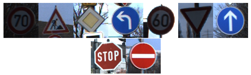
To build our classifier, we will use the German Traffic Sign Benchmark (GTSRB) (https://benchmark.ini.rub.de/) a multi-class, single-image classification challenge held at the International Joint Conference on Neural Networks (IJCNN) 2011.
This benchmark has the following properties:
Single-image, multi-class classification problem;
More than 40 classes;
More than 50,000 images in total;
Large, lifelike database.
Creation of the network
Defining the inputs of the Neural Network
First of all, if you have CUDA available, you can enable it with the following line :
n2d2.global_variables.default_model = "Frame_CUDA"
The default model is Frame.
Once this is done, you can load the database by using the appropriate driver n2d2.database.GTSRB.
We set 20% of the data to be used for validation.
To feed data to the network, you need to create a n2d2.provider.DataProvider this class will define the input fo neural network.
db = n2d2.database.GTSRB(0.2)
db.load(data_path) # Enter the path of your database !
provider = n2d2.provider.DataProvider(db, [29, 29, 1], batch_size=BATCH_SIZE)
You can apply pre-processing to the data with n2d2.transform.Transformation objects.
We have set the size of the input images to be 29x29 pixels with 1 channel when declaring the n2d2.provider.DataProvider.
But the dataset is composed of image of size comprised from 15x15 to 250x250 pixels with 3 channel (R,G,B).
We will add a n2d2.transform.Rescale to rescale the size of the image to be 29x29 pixels.
The other transformation n2d2.transform.ChannelExtraction will set the number of channel to 1 by creating images in nuance of grey.
provider.add_transformation(n2d2.transform.ChannelExtraction('Gray'))
provider.add_transformation(n2d2.transform.Rescale(width=29, height=29))
Defining the neural network
Now that we have defined the inputs, we can declare the neural network. We will create a network inspired from the well-known LeNet network.
Before we define the network, we will create default configuration for the different type of layer with n2d2.ConfigSection.
This will allow us to create cells more concisely. n2d2.ConfigSection are used like python dictionary.
solver_config = ConfigSection(
    learning_rate=0.01,
    momentum=0.9,
    decay=0.0005,
    learning_rate_decay=0.993)

fc_config   = ConfigSection(weights_filler=Xavier(),
                            no_bias=True,
                            weights_solver=SGD(**solver_config))
conv_config = ConfigSection(activation=Rectifier(),
                            weights_filler=Xavier(),
                            weights_solver=SGD(**solver_config),
                            no_bias=True)
For the ReLU activation function to be effective, the weights must be initialized carefully, in order to avoid dead units that would be stuck in the ]−∞,0] output range before the ReLU function. In N2D2, one can use a custom WeightsFiller for the weights initialization.
This is why we will use the n2d2.filler.Xavier algorithm to fill the weights of the different cells.
To define the network, we will use n2d2.cells.Sequence that take a list of n2d2.nn.NeuralNetworkCell.
model = n2d2.cells.Sequence([
    Conv(1, 32, [4, 4], **conv_config),
    Pool2d([2, 2], stride_dims=[2, 2], Pooling='Max'),
    Conv(32, 48, [5, 5], mapping=conv2_mapping, **conv_config),
    Pool2d([3, 3], stride_dims=[3, 3], Pooling='Max'),
    Fc(48*3*3, 200, activation=Rectifier(), **fc_config),
    Dropout(),
    Fc(200, 43, activation=Linear(), **fc_config),
    Softmax(with_loss=True)
])
Note that in LeNet, the conv2 layer is not fully connected to the Pooling layer.
In n2d2, a custom mapping can be defined for each input connection.
We can do this with the mapping argument by passing a n2d2.Tensor.
The connection of n-th output map to the inputs is defined by the n-th column of the matrix below, where the rows correspond to the inputs.
conv2_mapping=n2d2.Tensor([32, 48], datatype="bool")
conv2_mapping.set_values([
[1, 0, 0, 0, 0, 0, 0, 0, 0, 0, 0, 0, 0, 0, 0, 0, 0, 0, 0, 0, 0, 0, 0, 0, 0, 0, 0, 0, 0, 0, 0, 1, 0, 0, 0, 0, 0, 0, 0, 0, 0, 0, 0, 0, 0, 0, 1, 1],
[1, 1, 0, 0, 0, 0, 0, 0, 0, 0, 0, 0, 0, 0, 0, 0, 0, 0, 0, 0, 0, 0, 0, 0, 0, 0, 0, 0, 0, 0, 0, 1, 0, 0, 0, 0, 0, 0, 0, 0, 0, 0, 0, 0, 0, 0, 1, 1],
[0, 1, 1, 0, 0, 0, 0, 0, 0, 0, 0, 0, 0, 0, 0, 0, 0, 0, 0, 0, 0, 0, 0, 0, 0, 0, 0, 0, 0, 0, 0, 1, 1, 0, 0, 0, 0, 0, 0, 0, 0, 0, 0, 0, 0, 0, 1, 1],
[0, 0, 1, 1, 0, 0, 0, 0, 0, 0, 0, 0, 0, 0, 0, 0, 0, 0, 0, 0, 0, 0, 0, 0, 0, 0, 0, 0, 0, 0, 0, 1, 1, 0, 0, 0, 0, 0, 0, 0, 0, 0, 0, 0, 0, 0, 1, 1],
[0, 0, 0, 1, 1, 0, 0, 0, 0, 0, 0, 0, 0, 0, 0, 0, 0, 0, 0, 0, 0, 0, 0, 0, 0, 0, 0, 0, 0, 0, 0, 0, 1, 1, 0, 0, 0, 0, 0, 0, 0, 0, 0, 0, 0, 0, 1, 1],
[0, 0, 0, 0, 1, 1, 0, 0, 0, 0, 0, 0, 0, 0, 0, 0, 0, 0, 0, 0, 0, 0, 0, 0, 0, 0, 0, 0, 0, 0, 0, 0, 1, 1, 0, 0, 0, 0, 0, 0, 0, 0, 0, 0, 0, 0, 1, 1],
[0, 0, 0, 0, 0, 1, 1, 0, 0, 0, 0, 0, 0, 0, 0, 0, 0, 0, 0, 0, 0, 0, 0, 0, 0, 0, 0, 0, 0, 0, 0, 0, 0, 1, 1, 0, 0, 0, 0, 0, 0, 0, 0, 0, 0, 0, 1, 1],
[0, 0, 0, 0, 0, 0, 1, 1, 0, 0, 0, 0, 0, 0, 0, 0, 0, 0, 0, 0, 0, 0, 0, 0, 0, 0, 0, 0, 0, 0, 0, 0, 0, 1, 1, 0, 0, 0, 0, 0, 0, 0, 0, 0, 0, 0, 1, 1],
[0, 0, 0, 0, 0, 0, 0, 1, 1, 0, 0, 0, 0, 0, 0, 0, 0, 0, 0, 0, 0, 0, 0, 0, 0, 0, 0, 0, 0, 0, 0, 0, 0, 0, 1, 1, 0, 0, 0, 0, 0, 0, 0, 0, 0, 0, 1, 1],
[0, 0, 0, 0, 0, 0, 0, 0, 1, 1, 0, 0, 0, 0, 0, 0, 0, 0, 0, 0, 0, 0, 0, 0, 0, 0, 0, 0, 0, 0, 0, 0, 0, 0, 1, 1, 0, 0, 0, 0, 0, 0, 0, 0, 0, 0, 1, 1],
[0, 0, 0, 0, 0, 0, 0, 0, 0, 1, 1, 0, 0, 0, 0, 0, 0, 0, 0, 0, 0, 0, 0, 0, 0, 0, 0, 0, 0, 0, 0, 0, 0, 0, 0, 1, 1, 0, 0, 0, 0, 0, 0, 0, 0, 0, 1, 1],
[0, 0, 0, 0, 0, 0, 0, 0, 0, 0, 1, 1, 0, 0, 0, 0, 0, 0, 0, 0, 0, 0, 0, 0, 0, 0, 0, 0, 0, 0, 0, 0, 0, 0, 0, 1, 1, 0, 0, 0, 0, 0, 0, 0, 0, 0, 1, 1],
[0, 0, 0, 0, 0, 0, 0, 0, 0, 0, 0, 1, 1, 0, 0, 0, 0, 0, 0, 0, 0, 0, 0, 0, 0, 0, 0, 0, 0, 0, 0, 0, 0, 0, 0, 0, 1, 1, 0, 0, 0, 0, 0, 0, 0, 0, 1, 1],
[0, 0, 0, 0, 0, 0, 0, 0, 0, 0, 0, 0, 1, 1, 0, 0, 0, 0, 0, 0, 0, 0, 0, 0, 0, 0, 0, 0, 0, 0, 0, 0, 0, 0, 0, 0, 1, 1, 0, 0, 0, 0, 0, 0, 0, 0, 1, 1],
[0, 0, 0, 0, 0, 0, 0, 0, 0, 0, 0, 0, 0, 1, 1, 0, 0, 0, 0, 0, 0, 0, 0, 0, 0, 0, 0, 0, 0, 0, 0, 0, 0, 0, 0, 0, 0, 1, 1, 0, 0, 0, 0, 0, 0, 0, 1, 1],
[0, 0, 0, 0, 0, 0, 0, 0, 0, 0, 0, 0, 0, 0, 1, 1, 0, 0, 0, 0, 0, 0, 0, 0, 0, 0, 0, 0, 0, 0, 0, 0, 0, 0, 0, 0, 0, 1, 1, 0, 0, 0, 0, 0, 0, 0, 1, 1],
[0, 0, 0, 0, 0, 0, 0, 0, 0, 0, 0, 0, 0, 0, 0, 1, 1, 0, 0, 0, 0, 0, 0, 0, 0, 0, 0, 0, 0, 0, 0, 0, 0, 0, 0, 0, 0, 0, 1, 1, 0, 0, 0, 0, 0, 0, 1, 1],
[0, 0, 0, 0, 0, 0, 0, 0, 0, 0, 0, 0, 0, 0, 0, 0, 1, 1, 0, 0, 0, 0, 0, 0, 0, 0, 0, 0, 0, 0, 0, 0, 0, 0, 0, 0, 0, 0, 1, 1, 0, 0, 0, 0, 0, 0, 1, 1],
[0, 0, 0, 0, 0, 0, 0, 0, 0, 0, 0, 0, 0, 0, 0, 0, 0, 1, 1, 0, 0, 0, 0, 0, 0, 0, 0, 0, 0, 0, 0, 0, 0, 0, 0, 0, 0, 0, 0, 1, 1, 0, 0, 0, 0, 0, 1, 1],
[0, 0, 0, 0, 0, 0, 0, 0, 0, 0, 0, 0, 0, 0, 0, 0, 0, 0, 1, 1, 0, 0, 0, 0, 0, 0, 0, 0, 0, 0, 0, 0, 0, 0, 0, 0, 0, 0, 0, 1, 1, 0, 0, 0, 0, 0, 1, 1],
[0, 0, 0, 0, 0, 0, 0, 0, 0, 0, 0, 0, 0, 0, 0, 0, 0, 0, 0, 1, 1, 0, 0, 0, 0, 0, 0, 0, 0, 0, 0, 0, 0, 0, 0, 0, 0, 0, 0, 0, 1, 1, 0, 0, 0, 0, 1, 1],
[0, 0, 0, 0, 0, 0, 0, 0, 0, 0, 0, 0, 0, 0, 0, 0, 0, 0, 0, 0, 1, 1, 0, 0, 0, 0, 0, 0, 0, 0, 0, 0, 0, 0, 0, 0, 0, 0, 0, 0, 1, 1, 0, 0, 0, 0, 1, 1],
[0, 0, 0, 0, 0, 0, 0, 0, 0, 0, 0, 0, 0, 0, 0, 0, 0, 0, 0, 0, 0, 1, 1, 0, 0, 0, 0, 0, 0, 0, 0, 0, 0, 0, 0, 0, 0, 0, 0, 0, 0, 1, 1, 0, 0, 0, 1, 1],
[0, 0, 0, 0, 0, 0, 0, 0, 0, 0, 0, 0, 0, 0, 0, 0, 0, 0, 0, 0, 0, 0, 1, 1, 0, 0, 0, 0, 0, 0, 0, 0, 0, 0, 0, 0, 0, 0, 0, 0, 0, 1, 1, 0, 0, 0, 1, 1],
[0, 0, 0, 0, 0, 0, 0, 0, 0, 0, 0, 0, 0, 0, 0, 0, 0, 0, 0, 0, 0, 0, 0, 1, 1, 0, 0, 0, 0, 0, 0, 0, 0, 0, 0, 0, 0, 0, 0, 0, 0, 0, 1, 1, 0, 0, 1, 1],
[0, 0, 0, 0, 0, 0, 0, 0, 0, 0, 0, 0, 0, 0, 0, 0, 0, 0, 0, 0, 0, 0, 0, 0, 1, 1, 0, 0, 0, 0, 0, 0, 0, 0, 0, 0, 0, 0, 0, 0, 0, 0, 1, 1, 0, 0, 1, 1],
[0, 0, 0, 0, 0, 0, 0, 0, 0, 0, 0, 0, 0, 0, 0, 0, 0, 0, 0, 0, 0, 0, 0, 0, 0, 1, 1, 0, 0, 0, 0, 0, 0, 0, 0, 0, 0, 0, 0, 0, 0, 0, 0, 1, 1, 0, 1, 1],
[0, 0, 0, 0, 0, 0, 0, 0, 0, 0, 0, 0, 0, 0, 0, 0, 0, 0, 0, 0, 0, 0, 0, 0, 0, 0, 1, 1, 0, 0, 0, 0, 0, 0, 0, 0, 0, 0, 0, 0, 0, 0, 0, 1, 1, 0, 1, 1],
[0, 0, 0, 0, 0, 0, 0, 0, 0, 0, 0, 0, 0, 0, 0, 0, 0, 0, 0, 0, 0, 0, 0, 0, 0, 0, 0, 1, 1, 0, 0, 0, 0, 0, 0, 0, 0, 0, 0, 0, 0, 0, 0, 0, 1, 1, 1, 1],
[0, 0, 0, 0, 0, 0, 0, 0, 0, 0, 0, 0, 0, 0, 0, 0, 0, 0, 0, 0, 0, 0, 0, 0, 0, 0, 0, 0, 1, 1, 0, 0, 0, 0, 0, 0, 0, 0, 0, 0, 0, 0, 0, 0, 1, 1, 1, 1],
[0, 0, 0, 0, 0, 0, 0, 0, 0, 0, 0, 0, 0, 0, 0, 0, 0, 0, 0, 0, 0, 0, 0, 0, 0, 0, 0, 0, 0, 1, 1, 0, 0, 0, 0, 0, 0, 0, 0, 0, 0, 0, 0, 0, 0, 1, 1, 1],
[0, 0, 0, 0, 0, 0, 0, 0, 0, 0, 0, 0, 0, 0, 0, 0, 0, 0, 0, 0, 0, 0, 0, 0, 0, 0, 0, 0, 0, 0, 1, 0, 0, 0, 0, 0, 0, 0, 0, 0, 0, 0, 0, 0, 0, 1, 1, 1]])
After creating our network, we will create a n2d2.target.Target. This object will compute gradient and log training information that we will display later.
target = n2d2.target.Score(provider)
The n2d2.application.CrossEntropyClassifier deals with the output of the neural network, it computes the loss and propagates the gradient through the network.
Training the neural network
Once the neural network is defined, you can train it with the following loop :
for epoch in range(NB_EPOCH):
    print("\n\nEpoch : ", epoch)
    print("### Learning ###")
    provider.set_partition("Learn")
    model.learn()
    provider.set_reading_randomly(True)
    for stimuli in provider:
        output = model(stimuli)
        loss = target(output)
        loss.back_propagate()
        loss.update()
        print("Batch number : " + str(provider.batch_number()) + ", loss: " + "{0:.3f}".format(loss[0]), end='\r')
    print("\n### Validation ###")
    target.clear_success()
    provider.set_partition('Validation')
    model.test()
    for stimuli in provider:
        x = model(stimuli)
        x = target(x)
        print("Batch number : " + str(provider.batch_number()) + ", val success: "
                + "{0:.2f}".format(100 * target.get_average_success()) + "%", end='\r')
Once the learning phase is ended, you can test your network with the following loop :
print("\n### Testing ###")
provider.set_partition('Test')
model.test()
for stimuli in provider:
    x = model(stimuli)
    x = target(x)
    print("Batch number : " + str(provider.batch_number()) + ", test success: "
        + "{0:.2f}".format(100 * target.get_average_success()) + "%", end='\r')
print("\n")
Performance analysis tools
Once the training is done, you can log various statistics to analyze the performance of your network.
If you have done the testing loop you can use the following line to see the results :
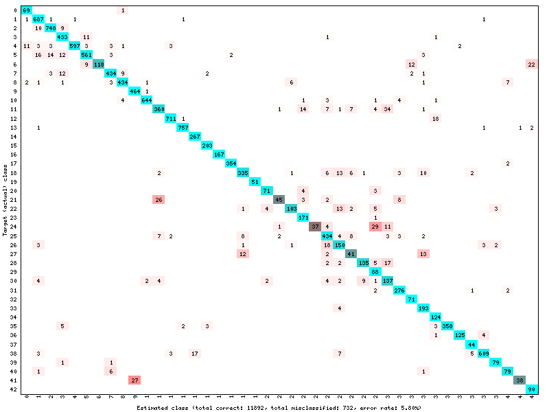
# save a confusion matrix
target.log_confusion_matrix("vis_GTSRB")
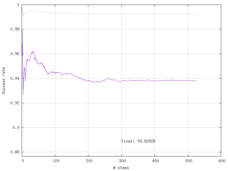
# save a graph of the loss and the validation score as a function of the number of steps
target.log_success("vis_GTSRB")
These methods will create images in a folder with the name of your Target. In this folder, you will find the confusion matrix :
And the training curve :
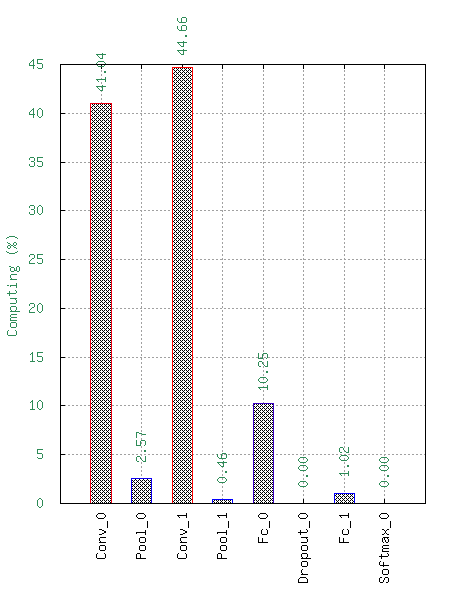
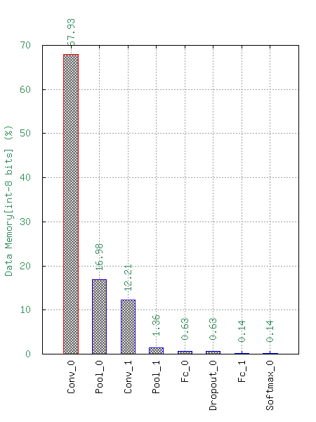
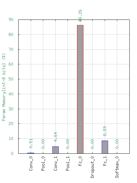
If you want to visualize the performance analysis of your neural network you can use the following line :
# save computational stats on the network
target.log_stats("vis_GTSRB")
This will generate the following statistics :
Number of Multiply-ACcumulate (MAC) operations per layers;
Number of parameters per layers;
Memory footprint per layers.
These data are available with a logarithm scale or a relative one.