Post-training quantization

Principle

The post-training quantization algorithm is done in 3 steps:

1) Weights normalization

All weights are rescaled in the range \([-1.0, 1.0]\).

Per layer normalization

There is a single weights scaling factor, global to the layer.

Per layer and per output channel normalization

There is a different weights scaling factor for each output channel. This allows a finer grain quantization, with a better usage of the quantized range for some output channels, at the expense of more factors to be saved in memory.

2) Activations normalization

Activations at each layer are rescaled in the range \([-1.0, 1.0]\) for signed outputs and \([0.0, 1.0]\) for unsigned outputs.

The optimal quantization threshold value of the activation output of each layer is determined using the validation dataset (or test dataset if no validation dataset is available).

This is an iterative process: need to take into account previous layers normalizing factors.

Finding the optimal quantization threshold value of the activation output of each layer is done the following:

1. Compute histogram of activation values;

2. Find threshold that minimizes distance between original distribution and clipped quantized distribution. Two distance algorithms can be used:

   • Mean Squared Error (MSE);

   • Kullback–Leibler divergence metric (KL-divergence).

   Another, simpler method, is to just clip the values above a fixed quantile.

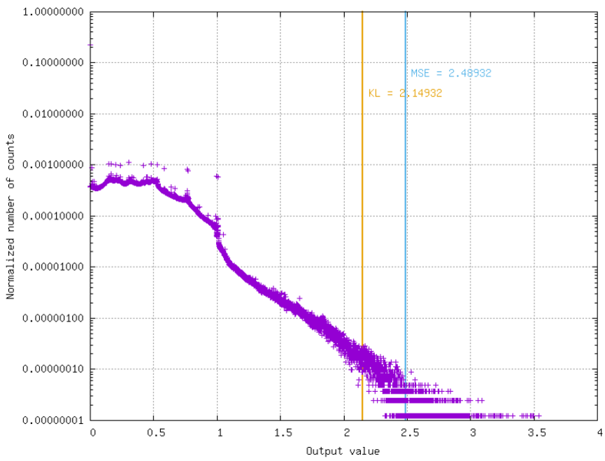
The obtained threshold value is therefore the activation scaling factor to be taken into account during quantization.

3) Quantization

Inputs, weights, biases and activations are quantized to the desired \(nbbits\) precision.

Convert ranges from \([-1.0, 1.0]\) and \([0.0, 1.0]\) to \([-2^{nbbits-1}-1, 2^{nbbits-1}-1]\) and \([0, 2^{nbbits}-1]\) taking into account all dependencies.

Additional optimization strategies

Weights clipping (optional)

Weights can be clipped using the same strategy than for the activations ( finding the optimal quantization threshold using the weights histogram). However, this usually leads to worse results than no clipping.

Activation scaling factor approximation

The activation scaling factor \(\alpha\) can be approximated the following ways:

• Fixed-point: \(\alpha\) is approximated by \(x 2^{-p}\);

• Single-shift: \(\alpha\) is approximated by \(2^{x}\);

• Double-shift: \(\alpha\) is approximated by \(2^{n} + 2^{m}\).

Usage in N2D2

All the post-training strategies described above are available in N2D2 for any export type. To apply post-training quantization during export, simply use the -calib command line argument.

The following parameters are available in command line:

Argument [default value]	Description
-calib	Number of stimuli used for the calibration (-1 = use the full validation dataset)
-calib-reload	Reload and reuse the data of a previous calibration
-wt-clipping-mode [None]	Weights clipping mode on export, can be None, MSE or KL-Divergence
-act-clipping-mode [MSE]	Activations clipping mode on export, can be None, MSE, KL-Divergence or Quantile
-act-rescaling-mode [Single-shift]	Activations scaling mode on export, can be Floating-point, Fixed-point16, Fixed-point32, Single-shift or Double-shift
-act-rescale-per-output [0]	If true (1), rescale activation per output instead of per layer
-act-quantile-value [0.9999]	If activation clipping mode is Quantile, fraction of the values to keep without clipping

-act-rescaling-mode

The -act-rescaling-mode specifies how the activation scaling must be approximated, for values other than Floating-point. This allows to avoid floating-point operation altogether in the generated code, even for complex, multi-branches networks. This is particularly useful on architectures without FPU or on FPGA.

For fixed-point scaling approximation (\(x 2^{-p}\)), two modes are available: Fixed-point16 and Fixed-point32. Fixed-point16 specifies that \(x\) must hold in at most 16-bits, whereas Fixed-point32 allows 32-bits \(x\). In the later case, beware that overflow can occur on 32-bits only architectures when computing the scaling multiplication before the right shift (\(p\)).

For the Single-shift and Double-shift modes, only right shifts are allowed (scaling factor < 1.0). In case of layers with scaling factor above 1.0, Fixed-point16 is used as fallback for these layers.

Command line example

Command line example to run the C++ Export on a INI file containing an ONNX model:

n2d2 MobileNet_ONNX.ini -seed 1 -w /dev/null -export CPP -fuse -calib -1 -act-clipping-mode KL-Divergence

With the python API

Examples and results

Post-training quantization accuracy obtained with some models from the ONNX Model Zoo are reported in the table below, using -calib 1000:

ONNX Model Zoo model (specificities)	FP acc.	Fake 8 bits acc.	8 bits acc.
resnet18v1.onnx (-no-unsigned -act-rescaling-mode Fixed-point)	69.83%	68.82%	68.78%
mobilenetv2-1.0.onnx (mobilenetv20_output_flatten0_reshape0 ignored)	70.95%	65.40%	65.40%
mobilenetv2-1.0.onnx (mobilenetv20_output_flatten0_reshape0 ignored -act-rescaling-mode Fixed-point)		66.67%	66.70%
squeezenet/model.onnx (-no-unsigned -act-rescaling-mode Floating-point)	57.58%	57.11%	54.98%

• FP acc. is the floating point accuracy obtained before post-training quantization on the model imported in ONNX;

• Fake 8 bits acc. is the accuracy obtained after post-training quantization in N2D2, in fake-quantized mode (the numbers are quantized but the representation is still floating point);

• 8 bits acc. is the accuracy obtained after post-training quantization in the N2D2 reference C++ export, in actual 8 bits representation.