Graph manipulation
In this example we will see :
How the N2D2 graph is generated;
How to draw the graph;
How to concatenate two Sequences;
How to get the output of a specific cell;
How to save only a certain part of the graph.
You can see the full script of this example here : graph_example.py.
For the following examples we will use the following objects :
fc1 = n2d2.cells.Fc(28*28, 50, activation=n2d2.activation.Rectifier())
fc2 = n2d2.cells.Fc(50, 10)
Printing n2d2 graph
The python API possess different vebosity level (default=`detailed`).
Short representation: only with compulsory constructor arguments
n2d2.global_variables.verbosity = n2d2.global_variables.Verbosity.short
print(fc1)
print(fc2)
Output :
'Fc_0' Fc(Frame<float>)(nb_inputs=784, nb_outputs=50)
'Fc_1' Fc(Frame<float>)(nb_inputs=50, nb_outputs=10)
Verbose representation: show graph and every arguments
n2d2.global_variables.verbosity = n2d2.global_variables.Verbosity.detailed
print(fc1)
print(fc2)
Output :
'Fc_0' Fc(Frame<float>)(nb_inputs=784, nb_outputs=50 | back_propagate=True, drop_connect=1.0, no_bias=False, normalize=False, outputs_remap=, weights_export_format=OC, activation=Rectifier(clipping=0.0, leak_slope=0.0, quantizer=None), weights_solver=SGD(clamping=, decay=0.0, iteration_size=1, learning_rate=0.01, learning_rate_decay=0.1, learning_rate_policy=None, learning_rate_step_size=1, max_iterations=0, min_decay=0.0, momentum=0.0, polyak_momentum=True, power=0.0, warm_up_duration=0, warm_up_lr_frac=0.25), bias_solver=SGD(clamping=, decay=0.0, iteration_size=1, learning_rate=0.01, learning_rate_decay=0.1, learning_rate_policy=None, learning_rate_step_size=1, max_iterations=0, min_decay=0.0, momentum=0.0, polyak_momentum=True, power=0.0, warm_up_duration=0, warm_up_lr_frac=0.25), weights_filler=Normal(mean=0.0, std_dev=0.05), bias_filler=Normal(mean=0.0, std_dev=0.05), quantizer=None)
'Fc_1' Fc(Frame<float>)(nb_inputs=50, nb_outputs=10 | back_propagate=True, drop_connect=1.0, no_bias=False, normalize=False, outputs_remap=, weights_export_format=OC, activation=None, weights_solver=SGD(clamping=, decay=0.0, iteration_size=1, learning_rate=0.01, learning_rate_decay=0.1, learning_rate_policy=None, learning_rate_step_size=1, max_iterations=0, min_decay=0.0, momentum=0.0, polyak_momentum=True, power=0.0, warm_up_duration=0, warm_up_lr_frac=0.25), bias_solver=SGD(clamping=, decay=0.0, iteration_size=1, learning_rate=0.01, learning_rate_decay=0.1, learning_rate_policy=None, learning_rate_step_size=1, max_iterations=0, min_decay=0.0, momentum=0.0, polyak_momentum=True, power=0.0, warm_up_duration=0, warm_up_lr_frac=0.25), weights_filler=Normal(mean=0.0, std_dev=0.05), bias_filler=Normal(mean=0.0, std_dev=0.05), quantizer=None)
Graph representation: show the object and the cell associated.
Note
Before propagation, no inputs are visible.
n2d2.global_variables.verbosity = n2d2.global_variables.Verbosity.graph_only
print(fc1)
print(fc2)
Output :
'Fc_0' Fc(Frame<float>)
'Fc_1' Fc(Frame<float>)
Now if we propagate a tensor to our cells, we will generate the computation graph and we will be able to see the linked cells :
x = n2d2.tensor.Tensor(dims=[1, 28, 28], value=0.5)

x = fc1(x)
x = fc2(x)
print(fc1)
print(fc2)
Output :
'Fc_0' Fc(Frame<float>)(['TensorPlaceholder_0'])
'Fc_1' Fc(Frame<float>)(['Fc_0'])
Now we can see the inputs object of each cells !
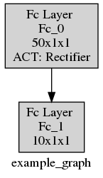
You can also plot the graph associated to a tensor with the method n2d2.Tensor.draw_associated_graph() :
x.draw_associated_graph("example_graph")
This will generate the following figure :
Manipulating Sequences
For this example we will show how you can use n2d2 to encapsulate Sequence.
We will create a LeNet and separate it two parts the extractor and the classifier.
from n2d2.cells import Sequence, Conv, Pool2d, Dropout, Fc
from n2d2.activation import Rectifier, Linear

extractor = Sequence([
    Conv(1, 6, kernel_dims=[5, 5]),
    Pool2d(pool_dims=[2, 2], stride_dims=[2, 2], pooling='Max'),
    Conv(6, 16, kernel_dims=[5, 5]),
    Pool2d(pool_dims=[2, 2], stride_dims=[2, 2], pooling='Max'),
    Conv(16, 120, kernel_dims=[5, 5]),
], name="extractor")

classifier = Sequence([
    Fc(120, 84, activation=Rectifier()),
    Dropout(dropout=0.5),
    Fc(84, 10, activation=Linear(), name="last_fully"),
], name="classifier")
We can concatenate these two sequences into one :
network = Sequence([extractor, classifier])

x = n2d2.Tensor([1,1,32,32], value=0.5)
output = network(x)

print(network)
Output
'Sequence_0' Sequence(
        (0): 'extractor' Sequence(
                (0): 'Conv_0' Conv(Frame<float>)(['TensorPlaceholder_1'])
                (1): 'Pool2d_0' Pool2d(Frame<float>)(['Conv_0'])
                (2): 'Conv_1' Conv(Frame<float>)(['Pool2d_0'])
                (3): 'Pool2d_1' Pool2d(Frame<float>)(['Conv_1'])
                (4): 'Conv_2' Conv(Frame<float>)(['Pool2d_1'])
        )
        (1): 'classifier' Sequence(
                (0): 'Fc_2' Fc(Frame<float>)(['Conv_2'])
                (1): 'Dropout_0' Dropout(Frame<float>)(['Fc_2'])
                (2): 'last_fully' Fc(Frame<float>)(['Dropout_0'])
        )
)
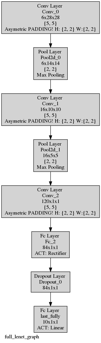
We can also plot the graph :
output.draw_associated_graph("full_lenet_graph")
We can also easily access the cells inside the encapsulated Sequence
first_fully = network["last_fully"]
print("Accessing the first fully connected layer which is encapsulated in a Sequence")
print(first_fully)
Output
'last_fully' Fc(Frame<float>)(['Dropout_0'])
This allow us for example to get the output of any cells after the propagation :
print(f"Output of the second fully connected : {first_fully.get_outputs()}")
Output
Output of the second fully connected : n2d2.Tensor([
[0][0]:
0.0135485
[1]:
0.0359611
[2]:
-0.0285292
[3]:
-0.0732218
[4]:
0.0318365
[5]:
-0.0930403
[6]:
0.0467896
[7]:
-0.108823
[8]:
0.0305202
[9]:
0.0055611
], device=cpu, datatype=f, cell='last_fully')
Concatenating n2d2.cells.Sequence can be useful if we want for example to only save the parameters of a part of the network.
network[0].export_free_parameters("ConvNet_parameters")
Output
Export to ConvNet_parameters/Conv_0.syntxt
Export to ConvNet_parameters/Conv_0_quant.syntxt
Export to ConvNet_parameters/Pool2d_0.syntxt
Export to ConvNet_parameters/Pool2d_0_quant.syntxt
Export to ConvNet_parameters/Conv_1.syntxt
Export to ConvNet_parameters/Conv_1_quant.syntxt
Export to ConvNet_parameters/Pool2d_1.syntxt
Export to ConvNet_parameters/Pool2d_1_quant.syntxt
Export to ConvNet_parameters/Conv_2.syntxt
Export to ConvNet_parameters/Conv_2_quant.syntxt