Quantization-Aware Training

Getting Started

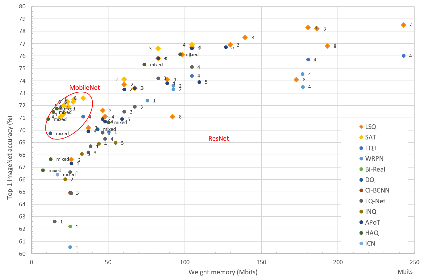
N2D2 provides a complete design environement for a super wide range of quantization modes. Theses modes are implemented as a set of integrated highly modular blocks. N2D2 implements a per layer quantization scheme that can be different at each level of the neural network. This high granularity enables to search for the best implementation depending on the hardware constraints. Moreover to achieve the best performances, N2D2 implements the latest quantization methods currently at the best of the state-of-the-art, summarized in the figure below. Each dot represents one DNN (from the MobileNet or ResNet family), quantized with the number of bits indicated beside.

The user can leverage the high modularity of our super set of quantizer blocks and simply choose the method that best fits with the initial requirements, computation resources and time to market strategy. For example to implement the LSQ method, one just need a limited number of training epochs to quantize a model while implementing the SAT method requires a higher number of training epochs but gives today the best quantization performance. In addition, the final objectives can be expressed in terms of different user requirements, depending on the compression capability of the targeted hardware. Depending on these different objectives we can consider different quantization schemes:

Weights-Only Quantization

In this quantization scheme only weights are discretized to fit in a limited set of possible states. Activations are not impacted. Let’s say we want to evaluate the performances of our model with 3 bits weights for convolutions layers. N2D2 natively provides the possibility to add a quantizer module, no need to import a new package or to modify any source code. We then just need to specify QWeight type and QWeight.Range for step level discretization.

...
QWeight=SAT ; Quantization Method can be ``LSQ`` or ``SAT``
QWeight.Range=15 ; Range is set to ``15`` step level, can be represented as a 4-bits word
...

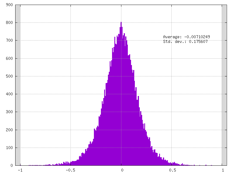
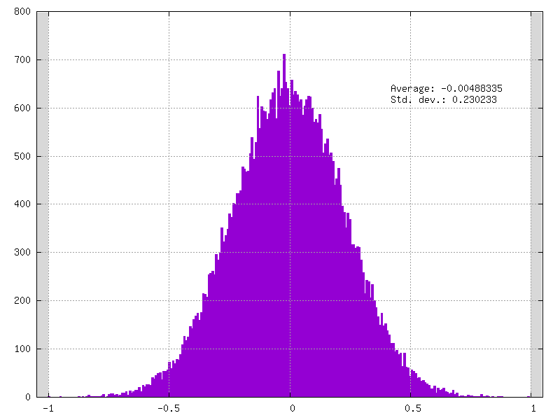
Example of fake-quantized weights on 4-bits / 15 levels:

Mixed Weights-Activations Quantization

In this quantization scheme both activations and weights are quantized at different possible step levels. For layers that have a non-linear activation function and learnable parameters, such as Fc and Conv, we first specify QWeight in the same way as Weights-Only quantization mode.

Let’s say now that we want to evaluate the performances of our model with activations quantized to 3-bits. In a similar manner, as for QWeight quantizer we specify the activation quantizer QAct for all layers that have a non-linear activation function. Where the method itself, here QAct=SAT ensures the non-linearity of the activation function.

...
ActivationFunction=Linear
QAct=SAT ; Quantization Method can be ``LSQ`` or ``SAT``
QAct.Range=7 ; Range is set to ``7`` step level, can be represented as a 3-bits word
...

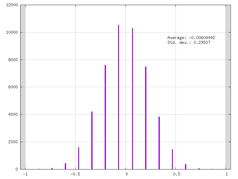
Example of an activation feature map quantized in 4-bits / 15 levels:

Integer-Only Quantization

Activations and weights are only represented as Integer during the learning phase, it’s one step beyond classical fake quantization !! In practice, taking advantage of weight-only quantization scheme or fake quantization is clearly not obvious on hardware components. The Integer-Only quantization mode is made to fill this void and enable to exploit QAT independently of the targeted hardware architecture. Most common programmable architectures like CPU, GPU, DSP can implement it without additional burden. In addition, hardware implementation like HLS or RTL description natively support low-precision integer operators. In this mode, we replace the default quantization mode of the weights as follows :

...
QWeight.Mode=Integer ; Can be ``Default`` (fake-quantization) mode or ``Integer``(true integer) mode
...

Example of full integer weights on 4-bits / 15 levels:

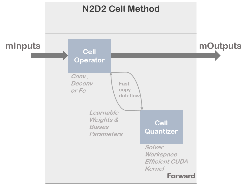
Cell Quantizer Definition

N2D2 implements a cell quantizer block for discretizing weights and biases at training time. This cell quantizer block is totally transparent for the user. The quantization phase of the learnable parameters requires intensive operation to adapt the distribution of the full-precision weights and to adapt the gradient. In addition the implementation can become highly memory greedy which can be a problem to train a complex model on a single GPU without specific treatment (gradient accumulation, etc..). That is why N2D2 merged different operations under dedicated CUDA kernels or CPU kernels allowing efficient utilization of available computation resources.

Overview of the cell quantizer implementation :

The common set of parameters for any kind of Cell Quantizer.

Option [default value]	Description
QWeight	Quantization method can be SAT or LSQ.
QWeight.Range [255]	Range of Quantization, can be 1 for binary, 255 for 8-bits etc..
QWeight.Solver [SGD]	Type of the Solver for learnable quantization parameters, can be SGD or ADAM
QWeight.Mode [Default]	Type of quantization Mode, can be Default or Integer

LSQ

The Learned Step size Quantization method is tailored to learn the optimal quantization step size parameters in parallel with the network weights. As described in [BLN+20], LSQ tries to estimate and scale the task loss gradient at each weight and activations layer’s quantizer step size, such that it can be learned in conjunction with other network parameters. This method can be initialized using weights from a pre-trained full precision model.

Option [default value]	Description
QWeight.StepSize [100]	Initial value of the learnable StepSize parameter
QWeight.StepOptInitStepSize [true]	If true initialize StepSize along first batch variance

SAT

Scale-Adjusted Training : [JYL19] method is one of the most promising solutions. The authors proposed SAT as a simple yet effective technique with which the rules of efficient training are maintained so that performance can be boosted and low-precision models can even surpass their full-precision counterparts in some cases. This method exploits DoReFa scheme for the weights quantization.

Option [default value]	Description
QWeight.ApplyQuantization [true]	Use true to enable quantization, if false parameters will be clamped between [-1.0,1.0]
QWeight.ApplyScaling [false]	Use true to scale the parameters as described in the SAT paper

Example of clamped weights when QWeight.ApplyQuantization=false:

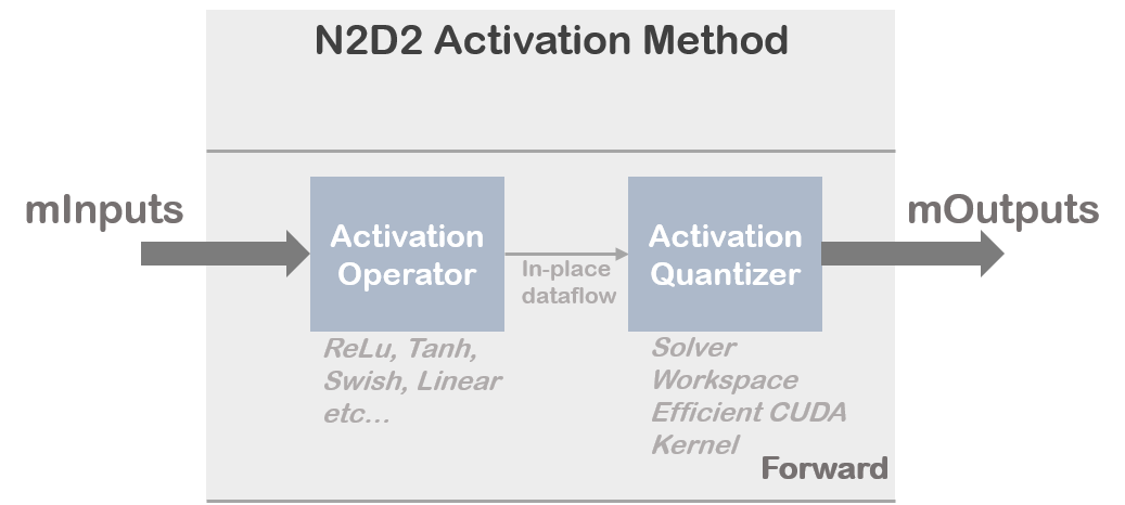
Activation Quantizer Definition

N2D2 implements an activation quantizer block to discretize activation at training time. Activation quantizer block is totally transparent for the user. Quantization phase of the activation requires intensive operation to learn parameters that will rescale the histogram of full-precision activation at training time. In addition the implementation can become highly memory greedy which can be a problem to train a complex model on a single GPU without specific treatment (gradient accumulation etc..). That why N2D2 merged different operations under dedicated CUDA kernels or CPU kernels allowing efficient utilization of available computing resources.

Overview of the activation quantizer implementation:

The common set of parameters for any kind of Activation Quantizer.

Option [default value]	Description
QAct	Quantization method can be SAT or LSQ.
QAct.Range [255]	Range of Quantization, can be 1 for binary, 255 for 8-bits etc..
QAct.Solver [SGD]	Type of the Solver for learnable quantization parameters, can be SGD or ADAM

LSQ

The Learned Step size Quantization method is tailored to learn the optimum quantization stepsize parameters in parallel to the network’s weights. As described in [BLN+20], LSQ tries to estimate and scale the task loss gradient at each weight and activations layer’s quantizer step size, such that it can be learned in conjunction with other network parameters. This method can be initialized using weights from a pre-trained full precision model.

Option [default value]	Description
QAct.StepSize [100]	Initial value of the learnable StepSize parameter
QAct.StepOptInitStepSize [true]	If true initialize StepSize following first batch variance

SAT

Scale-Adjusted Training : [JYL19] is one of the most promising solutions. The authors proposed SAT as a simple yet effective technique for which the rules of efficient training are maintained so that performance can be boosted and low-precision models can even surpass their full-precision counterparts in some cases. This method exploits a CG-PACT scheme for the activations quantization which is a boosted version of PACT for low precision quantization.

Option [default value]	Description
QAct.Alpha [8.0]	Initial value of the learnable alpha parameter

Layer compatibility table

Here we describe the compatibility table as a function of the quantization mode. The column Cell indicates layers that have a full support to quantize their learnable parameters during the training phase. The column Activation indicates layers that can support an activation quantizer to their output feature map. An additional column Integer Core indicates layers that can be represented without any full-precision operators at inference time. Of course it is necessary that their input comes from quantized activations.

Layer compatibility table	Quantization Mode
	Cell (parameters)	Activation	Integer Core
Activation		✓	✓
Anchor		✓	✗
BatchNorm*	✓	✓	✓
Conv	✓	✓	✓
Deconv	✓	✓	✓
ElemWise		✓	✓
Fc	✓	✓	✓
FMP		✓	✗
LRN	✗	✗	✗
LSTM	✗	✗	✗
ObjectDet		✓	✗
Padding		✓	✓
Pool		✓	✓
Proposal		✓	✗
Reshape		✓	✓
Resize		✓	✓
ROIPooling		✓	✗
RP		✓	✗
Scaling		✓	✓
Softmax		✓	✗
Threshold		✓	✓
Transformation		✓	✗
Transpose		✓	✓
Unpool		✓	✗

BatchNorm Cell parameters are not directly quantized during the training phase. N2D2 provides a unique approach to absorb its trained parameters as an integer within the only-integer representation of the network during a fusion phase. This method is guaranteed without any loss of applicative performances.

Tutorial

ONNX model : ResNet-18 Example - INI File

In this example we show how to quantize the resnet-18-v1 ONNX model with 4-bits weights and 4-bits activations using the SAT quantization method. We start from the resnet18v1.onnx file that you can pick-up at https://s3.amazonaws.com/onnx-model-zoo/resnet/resnet18v1/resnet18v1.onnx . You can also download it from the N2D2 script N2D2/tools/install_onnx_models.py that will automatically install a set of pre-trained ONNX models under your N2D2_MODELS system path.

Moreover you can start from .ini located at N2D2/models/ONNX/resnet-18-v1-onnx.ini and directly modify it or you can create an empty resnet18-v1.ini file in your simulation folder and to copy/paste all the following ini inistruction in it.

Also in this example you will need to know the ONNX cell names of your graph. We recommend you to opening the ONNX graph in a graph viewer like NETRON (https://lutzroeder.github.io/netron/).

In this example we focus to demonstrate how to apply SAT quantization procedure in the resnet-18-v1 ONNX model. The first step of the procedure consists to learn resnet-18-v1 on ImageNet database with clamped weights.

First of all we instantiate driver dataset and pre-processing / data augmentation function:

DefaultModel=Frame_CUDA
;ImageNet dataset
[database]
Type=ILSVRC2012_Database
RandomPartitioning=1
Learn=1.0

;Standard image resolution for ImageNet, batchsize=128
[sp]
SizeX=224
SizeY=224
NbChannels=3
BatchSize=128

[sp.Transformation-1]
Type=ColorSpaceTransformation
ColorSpace=RGB

[sp.Transformation-2]
Type=RangeAffineTransformation
FirstOperator=Divides
FirstValue=255.0

[sp.Transformation-3]
Type=RandomResizeCropTransformation
Width=224
Height=224
ScaleMin=0.2
ScaleMax=1.0
RatioMin=0.75
RatioMax=1.33
ApplyTo=LearnOnly

[sp.Transformation-4]
Type=RescaleTransformation
Width=256
Height=256
KeepAspectRatio=1
ResizeToFit=0
ApplyTo=NoLearn

[sp.Transformation-5]
Type=PadCropTransformation
Width=[sp.Transformation-4]Width
Height=[sp.Transformation-4]Height
ApplyTo=NoLearn

[sp.Transformation-6]
Type=SliceExtractionTransformation
Width=[sp]SizeX
Height=[sp]SizeY
OffsetX=16
OffsetY=16
ApplyTo=NoLearn

[sp.OnTheFlyTransformation-7]
Type=FlipTransformation
ApplyTo=LearnOnly
RandomHorizontalFlip=1

Now that dataset driver and pre-processing are well defined we can now focus on the neural network configuration. In our example we decide to quantize all convolutions and fully-connected layers. A base block common to all convolution layers can be defined in the .ini file. This specific base-block uses onnx:Conv_def that will overwrite the native definition of all convolution layers defined in the ONNX file. This base block is used to set quantization parameters, like weights bits range, the scaling mode and the quantization mode, and also solver configuration.

[onnx:Conv_def]
QWeight=SAT
QWeight.ApplyScaling=0  ; No scaling needed because each conv is followed by batch-normalization layers
QWeight.ApplyQuantization=0 ; Only clamp mode for the 1st step
WeightsFiller=XavierFiller ; Specific filler for SAT method
WeightsFiller.VarianceNorm=FanOut ; Specific filler for SAT method
WeightsFiller.Scaling=1.0 ; Specific filler for SAT method
ConfigSection=conv.config ; Config for conv parameters

[conv.config]
NoBias=1 ; No bias needed because each conv is followed by batch-normalization layers
Solvers.LearningRatePolicy=CosineDecay ; Can be different Policy following your problem, recommended with SAT method
Solvers.LearningRate=0.05 ; Typical value for batchsize=256 with SAT method
Solvers.Momentum=0.9 ; Typical value for batchsize=256 with SAT method
Solvers.Decay=0.00004 ; Typical value for batchsize=256 with SAT method
Solvers.MaxIterations=192175050; For 150-epoch on ImageNet 1 epoch = 1281167 samples, 150 epoch = 1281167*150 samples
Solvers.IterationSize=2 ;Our physical batch size is set to 128, iteration size is set to 2 because we want a batchsize of 256

A base block common to all Fully-Connected layers can be defined in the .ini file. This specific base-block uses onnx:Fc_def that will overwrite the native definition of all fully-connected layers defined in the ONNX file. This base block is used to set quantization parameters, like weights bits range, the scaling mode and the quantization mode, and also solver configuration.

[onnx:Fc_def]
QWeight=SAT
QWeight.ApplyScaling=1  ; Scaling needed for Full-Connected
QWeight.ApplyQuantization=0 ; Only clamp mode for the 1st step
WeightsFiller=XavierFiller ; Specific filler for SAT method
WeightsFiller.VarianceNorm=FanOut ; Specific filler for SAT method
WeightsFiller.Scaling=1.0 ; Specific filler for SAT method
ConfigSection=fc.config ; Config for conv parameters

[fc.config]
NoBias=0 ; Bias needed for fully-connected
Solvers.LearningRatePolicy=CosineDecay ; Can be different Policy following your problem, recommended with SAT method
Solvers.LearningRate=0.05 ; Typical value for batchsize=256 with SAT method
Solvers.Momentum=0.9 ; Typical value for batchsize=256 with SAT method
Solvers.Decay=0.00004 ; Typical value for batchsize=256 with SAT method
Solvers.MaxIterations=192175050; For 150-epoch on ImageNet 1 epoch = 1281167 samples, 150 epoch = 1281167*150 samples
Solvers.IterationSize=2 ;Our physical batch size is set to 128, iteration size is set to 2 because we want a batch size of 256

A base block common to all Batch-Normalization layers can be defined in the .ini file. This specific base-block uses onnx:Batchnorm_def that will overwrites the native definition of all the batch-normalization defined in the ONNX file. We simply defined here hyper-parameters of batch-normalization layers.

[onnx:BatchNorm_def]
ConfigSection=bn_train.config

[bn_train.config]
Solvers.LearningRatePolicy=CosineDecay ; Can be different Policy following your problem, recommended with SAT method
Solvers.LearningRate=0.05 ; Typical value for batchsize=256 with SAT method
Solvers.Momentum=0.9 ; Typical value for batchsize=256 with SAT method
Solvers.Decay=0.00004 ; Typical value for batchsize=256 with SAT method
Solvers.MaxIterations=192175050; For 150-epoch on ImageNet 1 epoch = 1281167 samples, 150 epoch = 1281167*150 samples
Solvers.IterationSize=2 ;Our physical batchsize is set to 128, iterationsize is set to 2 because we want a batchsize of 256

Then we described the resnet-18-v1 topology directly from the ONNX file that you previously installed in your simulation folder :

[onnx]
Input=sp
Type=ONNX
File=resnet18v1.onnx
ONNX_init=0 ; For SAT method we need to initialize from clamped weights or dedicated filler

[soft1]
Input=resnetv15_dense0_fwd
Type=Softmax
NbOutputs=1000
WithLoss=1

[soft1.Target]

Now that you set your resnet18-v1.ini file in your simulation folder you juste have to run the learning phase to clamp the weights with the command:

./n2d2 resnet18-v1.ini -learn-epoch 150 -valid-metric Precision

This command will run the learning phase over 150 epochs with the Imagenet dataset. The final test accuracy must reach at least 70%.

Next, you have to save parameters of the weights folder to the other location, for example weights_clamped folder.

Congratulations! Your resnet-18-v1 model have clamped weights now ! You can check the results in your weights_clamped folder. Now that your resnet-18-v1 model provides clamped weights you can play with it and try different quantization mode.

In addition, if you want to quantized also the resnet-18-v1 activations you need to create a specific base-block in your resnet-18-v1.ini file in that way :

[ReluQ_def]
ActivationFunction=Linear ; No more need Relu because SAT quantizer integrates it's own non-linear activation
QAct=SAT ; SAT quantization method
QAct.Range=15 ; Range=15 for 4-bits quantization model
QActSolver=SGD ; Specify SGD solver for learned alpha parameter
QActSolver.LearningRatePolicy=CosineDecay ; Can be different Policy following your problem, recommended with SAT method
QActSolver.LearningRate=0.05 ; Typical value for batchsize=256 with SAT method
QActSolver.Momentum=0.9 ; Typical value for batchsize=256 with SAT method
QActSolver.Decay=0.00004 ; Typical value for batchsize=256 with SAT method
QActSolver.MaxIterations=192175050; For 150-epoch on ImageNet 1 epoch = 1281167 samples, 150 epoch = 1281167*150 samples
QActSolver.IterationSize=2 ;Our physical batch size is set to 128, iteration size is set to 2 because we want a batchsize of 256

This base-block will be used to overwrites all the rectifier activation function of the ONNX model. To identify the name of the different activation function you can use the netron tool:

We then overrides all the activation function of the model by our previously described activation quantizer:

[resnetv15_relu0_fwd]ReluQ_def
[resnetv15_stage1_relu0_fwd]ReluQ_def
[resnetv15_stage1_activation0]ReluQ_def
[resnetv15_stage1_relu1_fwd]ReluQ_def
[resnetv15_stage1_activation1]ReluQ_def
[resnetv15_stage2_relu0_fwd]ReluQ_def
[resnetv15_stage2_activation0]ReluQ_def
[resnetv15_stage2_relu1_fwd]ReluQ_def
[resnetv15_stage2_activation1]ReluQ_def
[resnetv15_stage3_relu0_fwd]ReluQ_def
[resnetv15_stage3_activation0]ReluQ_def
[resnetv15_stage3_relu1_fwd]ReluQ_def
[resnetv15_stage3_activation1]ReluQ_def
[resnetv15_stage4_relu0_fwd]ReluQ_def
[resnetv15_stage4_activation0]ReluQ_def
[resnetv15_stage4_relu1_fwd]ReluQ_def
[resnetv15_stage4_activation1]ReluQ_def

Now that activations quantization mode is set we focuses on the weights parameters quantization. For example to quantize weights also in a 4 bits range, you should set the parameters convolution base-block in that way:

[onnx:Conv_def]
...
QWeight.ApplyQuantization=1 ; Set to 1 for quantization mode
QWeight.Range=15 ;  Conv is now quantized in 4-bits range (2^4 - 1)
...

In a same manner, you can modify the fully-connected base-block in that way :

[onnx:Fc_def]
...
QWeight.ApplyQuantization=1 ; Set to 1 for quantization mode
QWeight.Range=15 ;  Fc is now quantized in 4-bits range (2^4 - 1)
...

As a common practice in quantization aware training the first and last layers are quantized in 8-bits. In ResNet-18 the first layer is a convolution layer, we have to specify that to the first layer.

We first start to identify the name of the first layer under the netron environement:

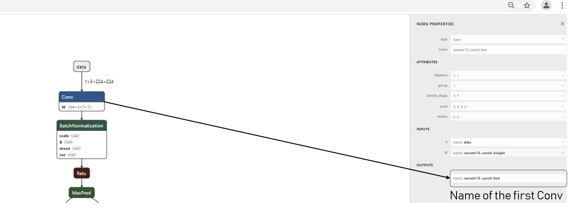
We then overrides the range of the first convolution layer of the resnet18v1.onnx model:

[resnetv15_conv0_fwd]onnx:Conv_def
QWeight.Range=255 ;resnetv15_conv0_fwd is now quantized in 8-bits range (2^8 - 1)

In a same way we overrides the range of the last fully-connected layer in 8-bits :

[resnetv15_dense0_fwd]onnx:Fc_def
QWeight.Range=255 ;resnetv15_dense0_fwd is now quantized in 8-bits range (2^8 - 1)

Now that your modified resnet-18-v1.ini file is ready just have to run a learning phase with the same hyperparameters by using transfer learning method from the previously clamped weights with this command:

./n2d2 resnet-18-v1.ini -learn-epoch 150 -w weights_clamped -valid-metric Precision

This command will run the learning phase over 150 epochs with the Imagenet dataset. The final test accuracy must reach at least 70%.

Congratulations! Your resnet-18-v1 model have now it’s weights parameters and activations quantized in a 4-bits way !

ONNX model : ResNet-18 Example - Python

In this example, we will do the same as in the previous section showcasing the python API.

You can find the complete scrip for this tutorial here resnet18v1 quantization example.

Firstly, you need to retrieved the resnet18v1.onnx file that you can pick-up at https://s3.amazonaws.com/onnx-model-zoo/resnet/resnet18v1/resnet18v1.onnx. Or with the N2D2 script N2D2/tools/install_onnx_models.py that will automatically install a set of pre-trained ONNX models under your N2D2_MODELS system path.

Once this is done, you can create a data provider for the dataset ILSVRC2012.

print("Create database")
database = n2d2.database.ILSVRC2012(learn=1.0, random_partitioning=True)
database.load(args.data_path, label_path=args.label_path)
print(database)
print("Create provider")
provider = n2d2.provider.DataProvider(database=database, size=[224, 224, 3], batch_size=batch_size)
print(provider)

We will then do some pre-processing to the data-set.

We use the n2d2.transform.Composite to have a compact syntax and avoid multiple call to the method add_transformation.

print("Adding transformations")
transformations = n2d2.transform.Composite([
    n2d2.transform.ColorSpace("RGB"),
    n2d2.transform.RangeAffine("Divides", 255.0),
    n2d2.transform.RandomResizeCrop(224, 224, scale_min=0.2, scale_max=1.0, ratio_min=0.75,
                                    ratio_max=1.33, apply_to="LearnOnly"),
    n2d2.transform.Rescale(256, 256, keep_aspect_ratio=True, resize_to_fit=False,
                          apply_to="NoLearn"),
    n2d2.transform.PadCrop(256, 256, apply_to="NoLearn"),
    n2d2.transform.SliceExtraction(224, 224, offset_x=16, offset_y=16, apply_to="NoLearn"),
])

print(transformations)

flip_trans = n2d2.transform.Flip(apply_to="LearnOnly", random_horizontal_flip=True)

provider.add_transformation(transformations)
provider.add_on_the_fly_transformation(flip_trans)
print(provider)

Once this is done, we can import the resnet-18-v1 ONNX model using n2d2.cells.DeepNetCell.

model = n2d2.cells.DeepNetCell.load_from_ONNX(provider, path_to_ONNX)

Once the ONNX model is loaded, we will change the configuration of the n2d2.cells.Conv, n2d2.cells.Fc and n2d2.cells.BatchNorm2d layers. To do so, we will iterate through the layer of our model and check the type of the layer. Then we will apply the wanted configuration for each cells.

print("Updating cells ...")

for cell in model:
    ### Updating Conv Cells ###
    if isinstance(cell, n2d2.cells.Conv):
        # You need to replace weights filler before adding the quantizer.
        cell.set_weights_filler(
            n2d2.filler.Xavier(
                variance_norm="FanOut",
                scaling=1.0,
        ), refill=True)

        if cell.has_bias():
            cell.refill_bias()
        cell.quantizer = SATCell(
                apply_scaling=False,
                apply_quantization=False
        )

        cell.set_solver_parameter("learning_rate_policy", "CosineDecay")
        cell.set_solver_parameter("learning_rate", 0.05)
        cell.set_solver_parameter("momentum", 0.9)
        cell.set_solver_parameter("decay", 0.00004)
        cell.set_solver_parameter("max_iterations", 192175050)
        cell.set_solver_parameter("iteration_size", 2)

    ### Updating Fc Cells ###
    if isinstance(cell, n2d2.cells.Fc):
        cell.set_weights_filler(
            n2d2.filler.Xavier(
                variance_norm="FanOut",
                scaling=1.0,
        ), refill=True)
        cell.set_bias_filler(
            n2d2.filler.Constant(
                value=0.0,
        ), refill=True)


        cell.quantizer = SATCell(
                apply_scaling=False,
                apply_quantization=False
        )
        cell.set_solver_parameter("learning_rate_policy", "CosineDecay")
        cell.set_solver_parameter("learning_rate", 0.05)
        cell.set_solver_parameter("momentum", 0.9)
        cell.set_solver_parameter("decay", 0.00004)
        cell.set_solver_parameter("max_iterations", 192175050)
        cell.set_solver_parameter("iteration_size", 2)

    ### Updating BatchNorm Cells ###
    if isinstance(cell, n2d2.cells.BatchNorm2d):
        cell.set_solver_parameter("learning_rate_policy", "CosineDecay")
        cell.set_solver_parameter("learning_rate", 0.05)
        cell.set_solver_parameter("momentum", 0.9)
        cell.set_solver_parameter("decay", 0.00004)
        cell.set_solver_parameter("max_iterations", 192175050)
        cell.set_solver_parameter("iteration_size", 2)
  print("AFTER MODIFICATION :")
  print(model)

Once this is done, we will do a regular training loop and save weights every time we met a new best precision during the validation phase. The clamped weights will be saved in a folder resnet_weights_clamped.

softmax = n2d2.cells.Softmax(with_loss=True)

loss_function =  n2d2.target.Score(provider)
max_precision = -1
print("\n### Training ###")
for epoch in range(nb_epochs):
    provider.set_partition("Learn")
    model.learn()

    print("\n# Train Epoch: " + str(epoch) + " #")

    for i in range(math.ceil(database.get_nb_stimuli('Learn') / batch_size)):
        x = provider.read_random_batch()
        x = model(x)
        x = softmax(x)
        x = loss_function(x)

        x.back_propagate()
        x.update()

        print("Example: " + str(i * batch_size) + ", loss: "
              + "{0:.3f}".format(x[0]), end='\r')

    print("\n### Validation ###")

    loss_function.clear_success()

    provider.set_partition('Validation')
    model.test()

    for i in range(math.ceil(database.get_nb_stimuli('Validation') / batch_size)):
        batch_idx = i * batch_size

        x = provider.read_batch(batch_idx)
        x = model(x)
        x = softmax(x)
        x = loss_function(x)

        print("Validate example: " + str(i * batch_size) + ", val success: "
              + "{0:.2f}".format(100 * loss_function.get_average_score(metric="Precision")) + "%", end='\r')

print("\nPloting the network ...")
x.get_deepnet().draw_graph("./resnet18v1_clamped")
x.get_deepnet().log_stats("./resnet18v1_clamped_stats")
print("Saving weights !")
model.get_embedded_deepnet().export_network_free_parameters("resnet_weights_clamped")

Your resnet-18-v1 model now have clamped weights !

Now we will change the quantizer objects to quantize the network et 4 bits (range=15).

print("Updating cells")

for cell in model:
    ### Updating Rectifier ###
    if isinstance(cell.activation, n2d2.activation.Rectifier):
        cell.activation = n2d2.activation.Linear(
                quantizer=SATAct(
                    range=15,
                    solver=n2d2.solver.SGD(
                        learning_rate_policy = "CosineDecay",
                        learning_rate=0.05,
                        momentum=0.9,
                        decay=0.00004,
                        max_iterations=115305030
        )))

    if isinstance(cell, (n2d2.cells.Conv, n2d2.cells.Fc)):
        cell.quantizer.set_quantization(True)
        cell.quantizer.set_range(15)

# The first and last cell are in 8 bits precision !
model["resnetv15_conv0_fwd"].quantizer.set_range(255)
model["resnetv15_dense0_fwd"].quantizer.set_range(255)

Once the quantizer objects have been updated we can run a new training loop to learn the quantized wieghts and activations.

print("\n### Training ###")
for epoch in range(nb_epochs):

    provider.set_partition("Learn")
    model.learn()

    print("\n# Train Epoch: " + str(epoch) + " #")

    for i in range(math.ceil(database.get_nb_stimuli('Learn') / batch_size)):
        x = provider.read_random_batch()
        x = model(x)
        x = softmax(x)
        x = loss_function(x)

        x.back_propagate()
        x.update()

        print("Example: " + str(i * batch_size) + ", loss: "
              + "{0:.3f}".format(x[0]), end='\r')

    print("\n### Validation ###")

    loss_function.clear_success()

    provider.set_partition('Validation')
    model.test()

    for i in range(math.ceil(database.get_nb_stimuli('Validation') / batch_size)):
        batch_idx = i * batch_size

        x = provider.read_batch(batch_idx)
        x = model(x)
        x = softmax(x)
        x = loss_function(x)

        print("Validate example: " + str(i * batch_size) + ", val success: "
              + "{0:.2f}".format(100 * loss_function.get_average_score(metric="Precision")) + "%", end='\r')

x.get_deepnet().draw_graph("./resnet18v1_quant")
x.get_deepnet().log_stats("./resnet18v1_quant_stats")
model.get_embedded_deepnet().export_network_free_parameters("resnet_weights_SAT")

You can look at your quantized weights in the newly created resnet_weights_SAT folder.

Hand-Made model : LeNet Example - INI File

One can apply the SAT quantization methodology on the chosen deep neural network by adding the right parameters to the .ini file. Here we show how to configure the .ini file to correctly apply the SAT quantization. In this example we decide to apply the SAT quantization procedure in a hand-made LeNet model. The first step of the procedure consists to learn LeNet on MNIST database with clamped weights.

We recommend you to create an empty LeNet.ini file in your simulation folder and to copy/paste all following ini block inside.

First of all we start to described MNIST driver dataset and pre-processing use for data augmentation at training and test phase:

; Frame_CUDA for GPU and Frame for CPU
DefaultModel=Frame_CUDA

; MNIST Driver Database Instantiation
[database]
Type=MNIST_IDX_Database
RandomPartitioning=1

; Environment Description , batch=256
[env]
SizeX=32
SizeY=32
BatchSize=256

[env.Transformation_0]
Type=RescaleTransformation
Width=32
Height=32

In our example we decide to quantize all convolutions and fully-connected layers. A base block common to all convolution layers can be defined in the .ini file. This base block is used to set quantization parameters, like weights bits range, the scaling mode and the quantization mode, and also solver configuration.

[Conv_def]
Type=Conv
ActivationFunction=Linear
QWeight=SAT
QWeight.ApplyScaling=0 ; No scaling needed because each conv is followed by batch-normalization layers
QWeight.ApplyQuantization=0 ; Only clamp mode for the 1st step
ConfigSection=common.config

[common.config]
NoBias=1
Solvers.LearningRate=0.05
Solvers.LearningRatePolicy=None
Solvers.Momentum=0.0
Solvers.Decay=0.0

A base block common to all Full-Connected layers can be defined in the .ini file. This base block is used to set quantization parameters, like weights bits range, the scaling mode and the quantization mode, and also solver configuration.

[Fc_def]
Type=Fc
ActivationFunction=Linear
QWeight=SAT
QWeight.ApplyScaling=1 ; Scaling needed because for Full-Conncted
QWeight.ApplyQuantization=0 ; Only clamp mode for the 1st step
ConfigSection=common.config

A base block common to all Batch-Normalization layers can be defined in the .ini file. This base block is used to set quantization activations, like activations bits range, the quantization mode, and also solver configuration. In this first step batch-normalization activation are not quantized yet. We simply defined a typical batch-normalization layer with Rectifier as non-linear activation function.

[Bn_def]
Type=BatchNorm
ActivationFunction=Rectifier
ConfigSection=bn.config

[bn.config]
Solvers.LearningRate=0.05
Solvers.LearningRatePolicy=None
Solvers.Momentum=0.0
Solvers.Decay=0.0

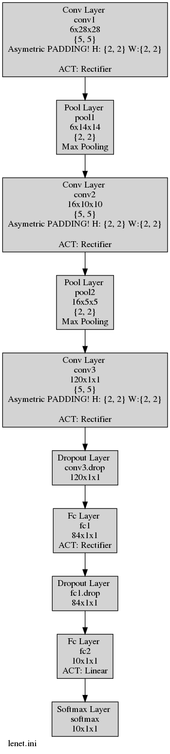
Finally we described the full backbone of LeNet topology:

[conv1] Conv_def
Input=env
KernelWidth=5
KernelHeight=5
NbOutputs=6

[bn1] Bn_def
Input=conv1
NbOutputs=[conv1]NbOutputs

; Non-overlapping max pooling P2
[pool1]
Input=bn1
Type=Pool
PoolWidth=2
PoolHeight=2
NbOutputs=6
Stride=2
Pooling=Max
Mapping.Size=1

[conv2] Conv_def
Input=pool1
KernelWidth=5
KernelHeight=5
NbOutputs=16
[bn2] Bn_def
Input=conv2
NbOutputs=[conv2]NbOutputs

[pool2]
Input=bn2
Type=Pool
PoolWidth=2
PoolHeight=2
NbOutputs=16
Stride=2
Pooling=Max
Mapping.Size=1

[conv3] Conv_def
Input=pool2
KernelWidth=5
KernelHeight=5
NbOutputs=120

[bn3]Bn_def
Input=conv3
NbOutputs=[conv3]NbOutputs

[conv3.drop]
Input=bn3
Type=Dropout
NbOutputs=[conv3]NbOutputs

[fc1] Fc_def
Input=conv3.drop
NbOutputs=84

[fc1.drop]
Input=fc1
Type=Dropout
NbOutputs=[fc1]NbOutputs

[fc2] Fc_def
Input=fc1.drop
ActivationFunction=Linear
NbOutputs=10

[softmax]
Input=fc2
Type=Softmax
NbOutputs=10
WithLoss=1

[softmax.Target]

Now that you have your ready LeNet.ini file in your simulation folder you juste have to run the learning phase to clamp the weights with the command:

./n2d2 LeNet.ini -learn-epoch 100

This command will run the learning phase over 100 epochs with the MNIST dataset. The final test accuracy must reach at least 98.9%:

Final recognition rate: 98.95%    (error rate: 1.05%)
Sensitivity: 98.94% / Specificity: 99.88% / Precision: 98.94%
Accuracy: 99.79% / F1-score: 98.94% / Informedness: 98.82%

Next, you have to save parameters of the weights folder to the other location, for example weights_clamped folder.

Congratulations! Your LeNet model have clamped weights now ! You can check the results in your weights_clamped folder, for example check your conv3_weights_quant.distrib.png file :

Now that your LeNet model provides clamped weights you can play with it and try different quantization mode. Moreover, if you want to quantized also the LeNet activations you have to modify the batch-normalization base-block from your LeNet.ini file in that way :

[Bn_def]
Type=BatchNorm
ActivationFunction=Linear ; Replace by linear: SAT quantizer directly apply non-linear activation
QAct=SAT
QAct.Alpha=6.0
QAct.Range=15 ; ->15 for 4-bits range (2^4 - 1)
QActSolver=SGD
QActSolver.LearningRate=0.05
QActSolver.LearningRatePolicy=None
QActSolver.Momentum=0.0
QActSolver.Decay=0.0
ConfigSection=bn.config

For example to quantize weights also in a 4 bits range, these parameters from the convolution base-block must be modified in that way:

[Conv_def]
Type=Conv
ActivationFunction=Linear
QWeight=SAT
QWeight.ApplyScaling=0
QWeight.ApplyQuantization=1 ; ApplyQuantization is now set to 1
QWeight.Range=15 ; Conv is now quantized in 4-bits range (2^4 - 1)
ConfigSection=common.config

In the same way, you have to modify the fully-connected base-block:

[Fc_def]
Type=Fc
ActivationFunction=Linear
QWeight=SAT
QWeight.ApplyScaling=1
QWeight.ApplyQuantization=1 ; ApplyQuantization is now set to 1
QWeight.Range=15 ; FC is now quantized in 4-bits range (2^4 - 1)
ConfigSection=common.config

As a common practice, the first and last layer are kept with 8-bits range weights parameters. To do that, the first conv1 layer of the LeNet backbone must be modified in that way:

[conv1] Conv_def
Input=env
KernelWidth=5
KernelHeight=5
NbOutputs=6
QWeight.Range=255 ; conv1 is now quantized in 8-bits range (2^8 - 1)

And the last layer fc2 of the LeNet must be modified in that way:

[fc2] Fc_def
Input=fc1.drop
ActivationFunction=Linear
NbOutputs=10
QWeight.Range=255 ; FC is now quantized in 8-bits range (2^8 - 1)

Now that your modified LeNet.ini file is ready just have to run a learning phase with the same hyperparameters by using transfer learning method from the previously clamped weights with this command:

./n2d2 LeNet.ini -learn-epoch 100 -w weights_clamped

The final test accuracy should be close to 99%:

Final recognition rate: 99.18%    (error rate: 0.82%)
  Sensitivity: 99.173293% / Specificity: 99.90895% / Precision: 99.172422%
  Accuracy: 99.836% / F1-score: 99.172195% / Informedness: 99.082242%

Congratulations! Your LeNet model is now fully-quantized ! You can check the results in your weights folder, for example check your conv3_weights_quant.distrib.png file :

In addition you can have your model graph view that integrates the quantization information. This graph is automatically generated at the learning phase or at the test phase. In this example this graph is generated under the name LeNet.ini.png.

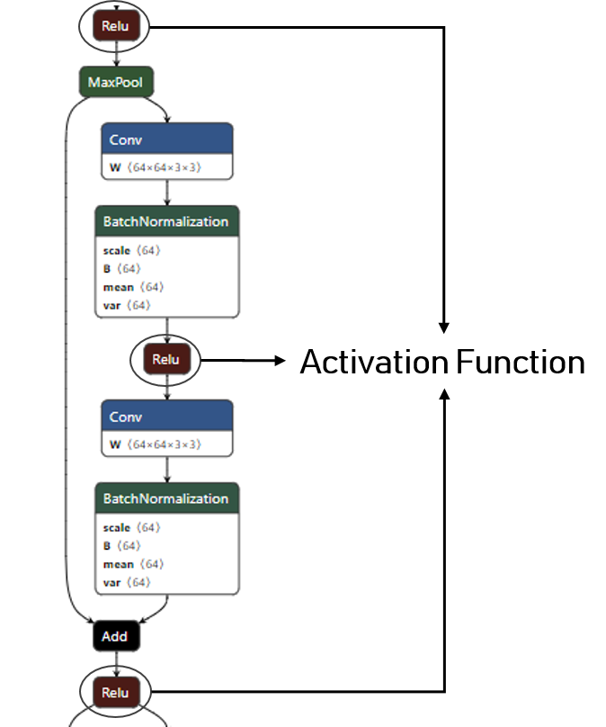
As you can see in the following figure, the batch-normalization layers are present (and essential) in your quantized model:

Obviously, no one wants batch-normalization layers in it’s quantized model. We answer this problem with our internal tool named DeepNetQAT. This tool allowed us to fused batch normalization parameters within the scaling, clipping and biases parameters of our quantized models under the SAT method.

You can fuse the batch normalization parameters of your model with this command :

./n2d2 LeNet.ini -test -qat-sat -w weights

Results must be exactly the same than with batch-normalization. Moreover quantizer modules have been entirely removed from your model ! You can check the results in the newly generated LeNet.ini.png graph :

Moreover you can find your quantized weights and biases under the folder weights_quantized.

Hand-Made model : LeNet Example - Python

Part 1 : Learn with clamped weights

In this section, we will see how to apply the SAT quantization methodology using the python API. We will apply the SAT quantization procedure in a handmade LeNet model.

You can get the script used in this example by clicking here : LeNet quantization example.

The first step is to learn LeNet on MNIST database with clamped weights.

Let’s start by importing the folowing libraries and setting some global variables :

import n2d2
import n2d2_ip
from n2d2.cells.nn import Dropout, Fc, Conv, Pool2d, BatchNorm2d
import math

nb_epochs = 100
batch_size = 256
n2d2.global_variables.cuda_device = 2
n2d2.global_variables.default_model = "Frame_CUDA"

Let’s create a database driver for MNIST, a dataprovider and apply transformation to the data.

print("\n### Create database ###")
database = n2d2.database.MNIST(data_path=data_path, validation=0.1)
print(database)
print("\n### Create Provider ###")
provider = n2d2.provider.DataProvider(database, [32, 32, 1], batch_size=batch_size)
provider.add_transformation(n2d2.transform.Rescale(width=32, height=32))
print(provider)

In our example we decided to quantize every convolutions and fully-connected layers. We will use the object n2d2.ConfigSection to provide common parameters to the cells.

Note

We need to use a function that will generate a new config section object to avoid giving the same objects to the one we are configuring. If we defined conv_conf as the solver_conf every Conv cells would have the same solver and quantizer object !

solver_conf = n2d2.ConfigSection(
    learning_rate=0.05,
    learning_rate_policy="None",
    momentum=0.0,
    decay=0.0,
)
def conv_conf():
    return n2d2.ConfigSection(
        activation=n2d2.activation.Linear(),
        no_bias=True,
        weights_solver=n2d2.solver.SGD(**solver_conf),
        bias_solver=n2d2.solver.SGD(**solver_conf),
        quantizer=n2d2_ip.quantizer.SATCell(
            apply_scaling=False, # No scaling needed because each conv is followed by batch-normalization layers
            apply_quantization=False, # Only clamp mode for the 1st step
    ),)
def fc_conf():
    return n2d2.ConfigSection(
        activation=n2d2.activation.Linear(),
        no_bias=True,
        weights_solver=n2d2.solver.SGD(**solver_conf),
        bias_solver=n2d2.solver.SGD(**solver_conf),
        quantizer=n2d2_ip.quantizer.SATCell(
            apply_scaling=True, # Scaling needed for Full-Connected
            apply_quantization=False, # Only clamp mode for the 1st step
        ),
    )
def bn_conf():
    return n2d2.ConfigSection(
        activation=n2d2.activation.Rectifier(),
        scale_solver=n2d2.solver.SGD(**solver_conf),
        bias_solver=n2d2.solver.SGD(**solver_conf),
    )

Once we have defined the global parameters for each cell, we can define our LeNet model.

print("\n### Loading Model ###")
model = n2d2.cells.Sequence([
    Conv(1, 6, kernel_dims=[5, 5], **conv_conf()),
    BatchNorm2d(6, **bn_conf()),
    Pool2d(pool_dims=[2, 2], stride_dims=[2, 2], pooling="Max"),
    Conv(6, 16, [5, 5], **conv_conf()),
    BatchNorm2d(16, **bn_conf()),
    Pool2d(pool_dims=[2, 2], stride_dims=[2, 2], pooling="Max"),
    Conv(16, 120, [5, 5], **conv_conf()),
    Dropout(name="Conv3.Dropout"),
    BatchNorm2d(120, **bn_conf()),
    Fc(120, 84, **fc_conf()),
    Dropout(name="Fc1.Dropout"),
    Fc(84, 10, **fc_conf()),
])
print(model)

softmax = n2d2.cells.Softmax(with_loss=True)

loss_function =  n2d2.target.Score(provider)

The model defined, we can train it with a classic training loop :

print("\n### Training ###")
for epoch in range(nb_epochs):

    provider.set_partition("Learn")
    model.learn()

    print("\n# Train Epoch: " + str(epoch) + " #")

    for i in range(math.ceil(database.get_nb_stimuli('Learn')/batch_size)):

        x = provider.read_random_batch()
        x = model(x)
        x = softmax(x)
        x = loss_function(x)
        x.back_propagate()
        x.update()

        print("Example: " + str(i * batch_size) + ", loss: "
              + "{0:.3f}".format(x[0]), end='\r')


    print("\n### Validation ###")

    loss_function.clear_success()

    provider.set_partition('Validation')
    model.test()

    for i in range(math.ceil(database.get_nb_stimuli('Validation') / batch_size)):
        batch_idx = i * batch_size

        x = provider.read_batch(batch_idx)
        x = model(x)
        x = softmax(x)
        x = loss_function(x)

        print("Validate example: " + str(i * batch_size) + ", val success: "
              + "{0:.2f}".format(100 * loss_function.get_average_success()) + "%", end='\r')


print("\n\n### Testing ###")

provider.set_partition('Test')
model.test()

for i in range(math.ceil(provider.get_database().get_nb_stimuli('Test')/batch_size)):
    batch_idx = i*batch_size

    x = provider.read_batch(batch_idx)
    x = model(x)
    x = softmax(x)
    x = loss_function(x)

    print("Example: " + str(i * batch_size) + ", test success: "
          + "{0:.2f}".format(100 * loss_function.get_average_success()) + "%", end='\r')

print("\n")

Then, we can export the weights we have learned in order to use them for the second step.

### Exporting weights ###
x.get_deepnet().export_network_free_parameters("./weights_clamped")

If you check the generated file : conv3_weights_quant.distrib.png you should see the clamped weights.

Part 2 : Quantized LeNet with SAT

Now that we have learned clamped weights, we will quantize our network.

You can get the script used in this example by clicking here : LeNet quantization example.

To do so, we will create a second script. We can begin by importing the MNIST database and create a dataprovider just like in the previous section.

Then we will copy the n2d2.ConfigSection from the previous section and add a quantizer argument.

solver_conf = n2d2.ConfigSection(
    learning_rate=0.05,
    learning_rate_policy="None",
    momentum=0.0,
    decay=0.0,
)
def conv_conf():
    return n2d2.ConfigSection(
        activation=n2d2.activation.Linear(),
        no_bias=True,
        weights_solver=n2d2.solver.SGD(**solver_conf),
        bias_solver=n2d2.solver.SGD(**solver_conf),
        quantizer=n2d2_ip.quantizer.SATCell(
            apply_scaling=False,
            apply_quantization=True, # ApplyQuantization is now set to True
            range=15, # Conv is now quantized in 4-bits range (2^4 - 1)
    ))
def fc_conf():
    return n2d2.ConfigSection(
        activation=n2d2.activation.Linear(),
        no_bias=True,
        weights_solver=n2d2.solver.SGD(**solver_conf),
        bias_solver=n2d2.solver.SGD(**solver_conf),
        quantizer=n2d2_ip.quantizer.SATCell(
            apply_scaling=True,
            apply_quantization=True, # ApplyQuantization is now set to True
            range=15, # Fc is now quantized in 4-bits range (2^4 - 1)
    ))
def bn_conf():
  return n2d2.ConfigSection(
      activation=n2d2.activation.Linear(
          quantizer=n2d2_ip.quantizer.SATAct(
              alpha=6.0,
              range=15, # -> 15 for 4-bits range (2^4-1)
      )),
      scale_solver=n2d2.solver.SGD(**solver_conf),
      bias_solver=n2d2.solver.SGD(**solver_conf),
  )

The configuration done, we will defined our new network.

Note

The first Convolution and last Fully Connected layer have differents parameters because we will quantize them in 8-bits instead of 4-bit as it is a common practice.

### Creating model ###
print("\n### Loading Model ###")
model = n2d2.cells.Sequence([
    Conv(1, 6, kernel_dims=[5, 5],
        activation=n2d2.activation.Linear(),
        no_bias=True,
        weights_solver=n2d2.solver.SGD(**solver_conf),
        bias_solver=n2d2.solver.SGD(**solver_conf),
        quantizer=n2d2_ip.quantizer.SATCell(
            apply_scaling=False,
            apply_quantization=True, # ApplyQuantization is now set to True
            range=255, # Conv_0 is now quantized in 8-bits range (2^8 - 1)
    )),
    BatchNorm2d(6, **bn_conf()),
    Pool2d(pool_dims=[2, 2], stride_dims=[2, 2], pooling="Max"),
    Conv(6, 16, [5, 5], **conv_conf()),
    BatchNorm2d(16, **bn_conf()),
    Pool2d(pool_dims=[2, 2], stride_dims=[2, 2], pooling="Max"),
    Conv(16, 120, [5, 5], **conv_conf()),
    Dropout(name="Conv3.Dropout"),
    BatchNorm2d(120, **bn_conf()),
    Fc(120, 84, **fc_conf()),
    Dropout(name="Fc1.Dropout"),
    Fc(84, 10,
        activation=n2d2.activation.Linear(),
        no_bias=True,
        weights_solver=n2d2.solver.SGD(**solver_conf),
        bias_solver=n2d2.solver.SGD(**solver_conf),
        quantizer=n2d2_ip.quantizer.SATCell(
            apply_scaling=True,
            apply_quantization=True, # ApplyQuantization is now set to True
            range=255, # Fc_1 is now quantized in 8-bits range (2^8 - 1)
    )),
])
print(model)

The model created we can import the learned parameter.

# Importing the clamped weights
model.import_free_parameters("./weights_clamped", ignore_not_exists=True)

The model is now ready for a training (you can use the training loop presented in the previous section).

The training done, you can save the new quantized weights with the following line :

### Exporting weights ###
x.get_deepnet().export_network_free_parameters("./new_weights")

If you check the generated file : conv3_weights_quant.distrib.png you should see the quantize weights.

You can fuse BatchNorm and Conv layers by using the following line :

### Fuse ###
n2d2_ip.quantizer.fuse_qat(x.get_deepnet(), provider, "NONE")
x.get_deepnet().draw_graph("./lenet_quant.py")

You can check the generated file : lenet_quant.py.png which should looks like the fig QAT without Batchnorm.

Results

Training Time Performances

Quantization-aware training induces intensive operations at training phase. Forward and backward phases require a lot of additional arithmetic operations compared to the standard floating-point training. The cost of operations involved in quantization-aware training method directly impacts the training time of a model.

To mitigate this loss at training time, that can be a huge handicap to quantize your own model, N2D2 implements CUDA kernels to efficiently perform these additional operations.

Here we estimate the training time per epoch for several well-known models on ImageNet and CIFAR-100 datasets. These data are shared for information purpose, to give you a realistic idea of the necessary time required to quantize your model. It relies on a lot of parameters like the dimension of your input data, the size of your dataset, pre-processing, your server/computer set-up installation, etc…

ResNet-18 Per Epoch Training Time
Quantization Method - Database	GPU Configuration
	A100 x1	2080 RTX Ti x1
SAT - ImageNet	15 min	40 min
SAT - CIFAR100	20 sec	1:15 min
LSQ - ImageNet	15 min	55 min

MobileNet-v1 Per Epoch Training Time
Quantization Method - Database	GPU Configuration
	A100 x1	2080 RTX Ti x1
SAT - ImageNet	25 min	45 min
SAT - CIFAR100	30 sec	1:30 min

MobileNet-v2 Per Epoch Training Time
Quantization Method - Database	GPU Configuration
	A100 x1	2080 RTX Ti x1
SAT - ImageNet	30 min	62 min
SAT - CIFAR100	1:15 min	2:10 min
LSQ - ImageNet	33 min	xx min

Inception-v1 Per Epoch Training Time
Quantization Method - Database	GPU Configuration
	A100 x1	2080 RTX Ti x1
SAT - ImageNet	40 min	80 min
SAT - CIFAR100	35 sec	2:20 min
LSQ - ImageNet	25 min	xx min

These performances indicators have been realized with typical Float32 datatype. Even if most of the operations used in the quantizations methods provides support for Float16 (half-precision) datatypes we recommend to not use it. In our experiments we observes performances differences compared to the Float32 datatype mode. These differences comes from gradient instability when datatype is reduced to Float16.

MobileNet-v1

Results obtained with the SAT method (~150 epochs) under the integer only mode :

MobileNet-v1 - SAT ImageNet Performances - Integer ONLY
Top-1 Precision	Quantization Range (bits)		Parameters	Memory	Alpha
	Weights	Activations
72.60 %	8	8	4 209 088	4.2 MB	1.0
71.50 %	4	8	4 209 088	2.6 MB	1.0
65.00 %	2	8	4 209 088	1.8 MB	1.0
60.15 %	1	8	4 209 088	1.4 MB	1.0
70.90 %	4	4	4 209 088	2.6 MB	1.0
64.60 %	3	3	4 209 088	2.2 MB	1.0
57.00 %	2	2	4 209 088	1.8 MB	1.0
69.00 %	8	8	3 156 816	2.6 MB	0.75
69.00 %	4	8	3 156 816	1.6 MB	0.75
65.60 %	3	8	3 156 816	1.4 MB	0.75
58.70 %	2	8	3 156 816	1.2 MB	0.75
53.80 %	1	8	3 156 816	0.9 MB	0.75
64.70 %	8	8	1 319 648	1.3 MB	0.5
63.40 %	4	8	1 319 648	0.9 MB	0.5
51.70 %	2	8	1 319 648	0.7 MB	0.5
44.00 %	1	8	1 319 648	0.6 MB	0.5
63.70 %	4	4	1 319 648	0.9 MB	0.5
54.80 %	3	3	1 319 648	0.8 MB	0.5
42.80 %	2	2	1 319 648	0.7 MB	0.5
55.01 %	8	8	463 600	0.4 MB	0.25
50.02 %	4	8	463 600	0.3 MB	0.25
46.80 %	3	8	463 600	0.3 MB	0.25
48.80 %	4	4	463 600	0.3 MB	0.25

MobileNet-v2

Results obtained with the SAT method (~150 epochs) under the integer only mode :

MobileNet-v2 - SAT ImageNet Performances - Integer ONLY
Top-1 Precision	Quantization Range (bits)		Parameters	Memory	Alpha
	Weights	Activations
72.5 %	8	8	3 214 048	3.2 MB	1.0
58.59 %	1	8	3 214 048	1.3 MB	1.0
70.93 %	4	4	3 214 048	2.1 MB	1.0

Results obtained with the LSQ method on 1 epoch :

MobileNet-v2 - LSQ ImageNet Performances - 1-Epoch
Top-1 Precision	Quantization Range (bits)		Parameters	Memory	Alpha
	Weights	Activations
70.1 %	8	8	3 214 048	3.2 MB	1.0

ResNet

Results obtained with the SAT method (~150 epochs) under the integer only mode :

ResNet - SAT ImageNet Performances - Integer ONLY
Top-1 Precision	Quantization Range (bits)		Parameters	Memory	Depth
	Weights	Activations
70.80 %	8	8	11 506 880	11.5 MB	18
67.6 %	1	8	11 506 880	1.9 MB	18
70.00 %	4	4	11 506 880	6.0 MB	18

Results obtained with the LSQ method on 1 epoch :

ResNet - LSQ ImageNet Performances - 1-Epoch
Top-1 Precision	Quantization Range (bits)		Parameters	Memory	Depth
	Weights	Activations
70.20 %	8	8	11 506 880	11.5 MB	18

Inception-v1

Results obtained with the SAT method (~150 epochs) under the integer only mode :

Inception-v1 - SAT ImageNet Performances - Integer ONLY
Top-1 Precision	Quantization Range (bits)		Parameters	Memory
	Weights	Activations
73.60 %	8	8	6 600 006	6.6 MB
68.60 %	1	8	6 600 006	1.7 MB
72.30 %	4	4	6 600 006	3.8 MB
68.50 %	1	4	6 600 006	1.7 MB
67.50 %	1	3	6 600 006	1.7 MB
63.30 %	1	2	6 600 006	1.7 MB
47.36 %	1	1	6 600 006	1.7 MB

Results obtained with the LSQ method on 1 epoch :

Inception-v1 - LSQ ImageNet Performances - 1-Epoch
Top-1 Precision	Quantization Range (bits)		Parameters	Memory
	Weights	Activations
72.60 %	8	8	6 600 006	6.6 MB