Tutorials
Learning deep neural networks: tips and tricks
Choose the learning solver
Generally, you should use the SGD solver with a momemtum (typical value for the momentum: 0.9). It generalizes better, often significantly better, than adaptive methods like Adam [WilsonRoelofsStern+17].
Adaptive solvers, like Adam, may be used for fast exploration and prototyping, thanks to their fast convergence.
Choose the learning hyper-parameters
You can use the -find-lr option available in the n2d2 executable
to automatically find the best learning rate for a given neural network.
Usage example:
./n2d2 model.ini -find-lr 10000
This command starts from a very low learning rate (1.0e-6) and increase it exponentially to reach the maximum value (10.0) after 10000 steps, as shown in figure [fig:findLrRange]. The loss change during this phase is then plotted in function of the learning rate, as shown in figure [fig:findLr].
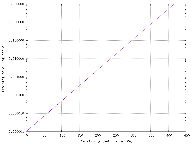
Exponential increase of the learning rate over the specified number of iterations, equals to the number of steps divided by the batch size (here: 24).
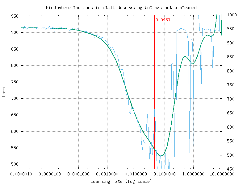
Loss change as a function of the learning rate.
Note that in N2D2, the learning rate is automatically normalized by the
global batch size (\(N \times \text{\lstinline!IterationSize!}\))
for the SGDSolver. A simple linear scaling rule is used, as
recommanded in [GDollarG+17].
The effective learning rate \(\alpha_{\text{eff}}\) applied for
parameters update is therefore:
Typical values for the SGDSolver are:
Solvers.LearningRate=0.01
Solvers.Decay=0.0001
Solvers.Momentum=0.9
Convergence and normalization
Deep networks (> 30 layers) and especially residual networks usually don’t converge without normalization. Indeed, batch normalization is almost always used. ZeroInit is a method that can be used to overcome this issue without normalization [ZDM19].
Building a classifier neural network
For this tutorial, we will use the classical MNIST handwritten digit
dataset. A driver module already exists for this dataset, named
MNIST_IDX_Database.
To instantiate it, just add the following lines in a new INI file:
[database]
Type=MNIST_IDX_Database
Validation=0.2 ; Use 20\% of the dataset for validation
In order to create a neural network, we first need to define its input,
which is declared with a [sp] section (sp for StimuliProvider).
In this section, we configure the size of the input and the batch size:
[sp]
SizeX=32
SizeY=32
BatchSize=128
We can also add pre-processing transformations to the StimuliProvider,
knowing that the final data size after transformations must match the
size declared in the [sp] section. Here, we must rescale the MNIST
28x28 images to match the 32x32 network input size.
[sp.Transformation_1]
Type=RescaleTransformation
Width=[sp]SizeX
Height=[sp]SizeY
Next, we declare the neural network layers. In this example, we reproduced the well-known LeNet network. The first layer is a 5x5 convolutional layer, with 6 channels. Since there is only one input channel, there will be only 6 convolution kernels in this layer.
[conv1]
Input=sp
Type=Conv
KernelWidth=5
KernelHeight=5
NbOutputs=6
The next layer is a 2x2 MAX pooling layer, with a stride of 2 (non-overlapping MAX pooling).
[pool1]
Input=conv1
Type=Pool
PoolWidth=2
PoolHeight=2
NbOutputs=[conv1]NbOutputs
Stride=2
Pooling=Max
Mapping.Size=1 ; One to one connection between input and output channels
The next layer is a 5x5 convolutional layer with 16 channels.
[conv2]
Input=pool1
Type=Conv
KernelWidth=5
KernelHeight=5
NbOutputs=16
Note that in LeNet, the [conv2] layer is not fully connected to the
pooling layer. In N2D2, a custom mapping can be defined for each input
connection. The connection of \(n\)-th output map to the inputs is
defined by the \(n\)-th column of the matrix below, where the rows
correspond to the inputs.
Mapping(pool1)=\
1 0 0 0 1 1 1 0 0 1 1 1 1 0 1 1 \
1 1 0 0 0 1 1 1 0 0 1 1 1 1 0 1 \
1 1 1 0 0 0 1 1 1 0 0 1 0 1 1 1 \
0 1 1 1 0 0 1 1 1 1 0 0 1 0 1 1 \
0 0 1 1 1 0 0 1 1 1 1 0 1 1 0 1 \
0 0 0 1 1 1 0 0 1 1 1 1 0 1 1 1
Another MAX pooling and convolution layer follow:
[pool2]
Input=conv2
Type=Pool
PoolWidth=2
PoolHeight=2
NbOutputs=[conv2]NbOutputs
Stride=2
Pooling=Max
Mapping.Size=1

[conv3]
Input=pool2
Type=Conv
KernelWidth=5
KernelHeight=5
NbOutputs=120
The network is composed of two fully-connected layers of 84 and 10 neurons respectively:
[fc1]
Input=conv3
Type=Fc
NbOutputs=84

[fc2]
Input=fc1
Type=Fc
NbOutputs=10
Finally, we use a softmax layer to obtain output classification probabilities and compute the loss function.
[softmax]
Input=fc2
Type=Softmax
NbOutputs=[fc2]NbOutputs
WithLoss=1
In order to tell N2D2 to compute the error and the classification score
on this softmax layer, one must attach a N2D2 Target to this layer,
with a section with the same name suffixed with .Target:
[softmax.Target]
By default, the activation function for the convolution and the
fully-connected layers is the hyperbolic tangent. Because the [fc2]
layer is fed to a softmax, it should not have any activation function.
We can specify it by adding the following line in the [fc2] section:
[fc2]
...
ActivationFunction=Linear
In order to improve further the networks performances, several things can be done:
Use ReLU activation functions. In order to do so, just add the
following in the [conv1], [conv2], [conv3] and [fc1]
layer sections:
ActivationFunction=Rectifier
For the ReLU activation function to be effective, the weights must be
initialized carefully, in order to avoid dead units that would be stuck
in the \(]-\infty,0]\) output range before the ReLU function. In
N2D2, one can use a custom WeightsFiller for the weights
initialization. For the ReLU activation function, a popular and
efficient filler is the so-called XavierFiller (see the
[par:XavierFiller] section for more information):
WeightsFiller=XavierFiller
Use dropout layers. Dropout is highly effective to improve the
network generalization capacity. Here is an example of a dropout layer
inserted between the [fc1] and [fc2] layers:
[fc1]
...

[fc1.drop]
Input=fc1
Type=Dropout
NbOutputs=[fc1]NbOutputs

[fc2]
Input=fc1.drop ; Replaces "Input=fc1"
...
Tune the learning parameters. You may want to tune the learning rate and other learning parameters depending on the learning problem at hand. In order to do so, you can add a configuration section that can be common (or not) to all the layers. Here is an example of configuration section:
[conv1]
...
ConfigSection=common.config

[...]
...

[common.config]
NoBias=1
WeightsSolver.LearningRate=0.05
WeightsSolver.Decay=0.0005
Solvers.LearningRatePolicy=StepDecay
Solvers.LearningRateStepSize=[sp]_EpochSize
Solvers.LearningRateDecay=0.993
Solvers.Clamping=-1.0:1.0
For more details on the configuration parameters for the Solver, see
section [sec:WeightSolvers].
Add input distortion. See for example the
DistortionTransformation (section [par:DistortionTransformation]).
The complete INI model corresponding to this tutorial can be found in models/LeNet.ini.
In order to use CUDA/GPU accelerated learning, the default layer model
should be switched to Frame_CUDA. You can enable this model by
adding the following line at the top of the INI file (before the first
section):
DefaultModel=Frame_CUDA
Building a segmentation neural network
In this tutorial, we will learn how to do image segmentation with N2D2. As an example, we will implement a face detection and gender recognition neural network, using the IMDB-WIKI dataset.
First, we need to instanciate the IMDB-WIKI dataset built-in N2D2 driver:
[database]
Type=IMDBWIKI_Database
WikiSet=1 ; Use the WIKI part of the dataset
IMDBSet=0 ; Don't use the IMDB part (less accurate annotation)
Learn=0.90
Validation=0.05
DefaultLabel=background ; Label for pixels outside any ROI (default is no label, pixels are ignored)
We must specify a default label for the background, because we want to learn to differenciate faces from the background (and not simply ignore the background for the learning).
The network input is then declared:
[sp]
SizeX=480
SizeY=360
BatchSize=48
CompositeStimuli=1
In order to work with segmented data, i.e. data with bounding box
annotations or pixel-wise annotations (as opposed to a single label per
data), one must enable the CompositeStimuli option in the [sp]
section.
We can then perform various operations on the data before feeding it to the network, like for example converting the 3-channels RGB input images to single-channel gray images:
[sp.Transformation-1]
Type=ChannelExtractionTransformation
CSChannel=Gray
We must only rescale the images to match the networks input size. This
can be done using a RescaleTransformation, followed by a
PadCropTransformation if one want to keep the images aspect ratio.
[sp.Transformation-2]
Type=RescaleTransformation
Width=[sp]SizeX
Height=[sp]SizeY
KeepAspectRatio=1 ; Keep images aspect ratio

; Required to ensure all the images are the same size
[sp.Transformation-3]
Type=PadCropTransformation
Width=[sp]SizeX
Height=[sp]SizeY
A common additional operation to extend the learning set is to apply
random horizontal mirror to images. This can be achieved with the
following FlipTransformation:
[sp.OnTheFlyTransformation-4]
Type=FlipTransformation
RandomHorizontalFlip=1
ApplyTo=LearnOnly ; Apply this transformation only on the learning set
Note that this is an on-the-fly transformation, meaning it cannot be
cached and is re-executed every time even for the same stimuli. We also
apply this transformation only on the learning set, with the ApplyTo
option.
Next, the neural network can be described:
[conv1.1]
Input=sp
Type=Conv
...

[pool1]
...

[...]
...

[fc2]
Input=drop1
Type=Conv
...

[drop2]
Input=fc2
Type=Dropout
NbOutputs=[fc2]NbOutputs
A full network description can be found in the IMDBWIKI.ini file in the models directory of N2D2. It is a fully-CNN network.
Here we will focus on the output layers required to detect the faces and
classify their gender. We start from the [drop2] layer, which has
128 channels of size 60x45.
Faces detection
We want to first add an output stage for the faces detection. It is a 1x1 convolutional layer with a single 60x45 output map. For each output pixel, this layer outputs the probability that the pixel belongs to a face.
[fc3.face]
Input=drop2
Type=Conv
KernelWidth=1
KernelHeight=1
NbOutputs=1
Stride=1
ActivationFunction=LogisticWithLoss
WeightsFiller=XavierFiller
ConfigSection=common.config ; Same solver options that the other layers
In order to do so, the activation function of this layer must be of type
LogisticWithLoss.
We must also tell N2D2 to compute the error and the classification score
on this softmax layer, by attaching a N2D2 Target to this layer, with
a section with the same name suffixed with .Target:
[fc3.face.Target]
LabelsMapping=\${N2D2_MODELS}/IMDBWIKI_target_face.dat
; Visualization parameters
NoDisplayLabel=0
LabelsHueOffset=90
In this Target, we must specify how the dataset annotations are mapped
to the layer’s output. This can be done in a separate file using the
LabelsMapping parameter. Here, since the output layer has a single
output per pixel, the target value can only be 0 or 1. A target value of
-1 means that this output is ignored (no error back-propagated). Since
the only annotations in the IMDB-WIKI dataset are faces, the mapping
described in the IMDBWIKI_target_face.dat file is easy:
# background
background 0

# padding (*) is ignored (-1)
* -1

# not background = face
default 1
Gender recognition
We can also add a second output stage for gender recognition. Like before, it would be a 1x1 convolutional layer with a single 60x45 output map. But here, for each output pixel, this layer would output the probability that the pixel represents a female face.
[fc3.gender]
Input=drop2
Type=Conv
KernelWidth=1
KernelHeight=1
NbOutputs=1
Stride=1
ActivationFunction=LogisticWithLoss
WeightsFiller=XavierFiller
ConfigSection=common.config
The output layer is therefore identical to the face’s output layer, but the target mapping is different. For the target mapping, the idea is simply to ignore all pixels not belonging to a face and affect the target 0 to male pixels and the target 1 to female pixels.
[fc3.gender.Target]
LabelsMapping=\${N2D2_MODELS}/IMDBWIKI_target_gender.dat
; Only display gender probability for pixels detected as face pixels
MaskLabelTarget=fc3.face.Target
MaskedLabel=1
The content of the IMDBWIKI_target_gender.dat file would therefore look like:
# background
# ?-* (unknown gender)
# padding
default -1

# male gender
M-? 0   # unknown age
M-0 0
M-1 0
M-2 0
...
M-98 0
M-99 0

# female gender
F-? 1   # unknown age
F-0 1
F-1 1
F-2 1
...
F-98 1
F-99 1
ROIs extraction
The next step would be to extract detected face ROIs and assign for each ROI the most probable gender. To this end, we can first set a detection threshold, in terms of probability, to select face pixels. In the following, the threshold is fixed to 75% face probability:
[post.Transformation-thres]
Input=fc3.face
Type=Transformation
NbOutputs=1
Transformation=ThresholdTransformation
Operation=ToZero
Threshold=0.75
We can then assign a target of type TargetROIs to this layer that
will automatically create the bounding box using a segmentation
algorithm.
[post.Transformation-thres.Target-face]
Type=TargetROIs
MinOverlap=0.33 ; Min. overlap fraction to match the ROI to an annotation
FilterMinWidth=5 ; Min. ROI width
FilterMinHeight=5 ; Min. ROI height
FilterMinAspectRatio=0.5 ; Min. ROI aspect ratio
FilterMaxAspectRatio=1.5 ; Max. ROI aspect ratio
LabelsMapping=\${N2D2_MODELS}/IMDBWIKI_target_face.dat
In order to assign a gender to the extracted ROIs, the above target must be modified to:
[post.Transformation-thres.Target-gender]
Type=TargetROIs
ROIsLabelTarget=fc3.gender.Target
MinOverlap=0.33
FilterMinWidth=5
FilterMinHeight=5
FilterMinAspectRatio=0.5
FilterMaxAspectRatio=1.5
LabelsMapping=\${N2D2_MODELS}/IMDBWIKI_target_gender.dat
Here, we use the fc3.gender.Target target to determine the most
probable gender of the ROI.
Data visualization
For each Target in the network, a corresponding folder is created in the simulation directory, which contains learning, validation and test confusion matrixes. The output estimation of the network for each stimulus is also generated automatically for the test dataset and can be visualized with the ./test.py helper tool. An example is shown in figure [fig:targetvisu].
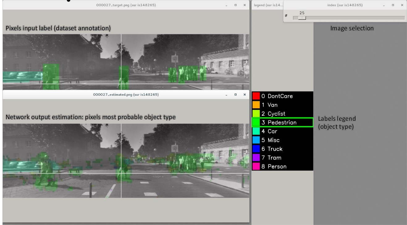
Example of the target visualization helper tool.
Transcoding a learned network in spike-coding
N2D2 embeds an event-based simulator (historically known as ’Xnet’) and allows to transcode a whole DNN in a spike-coding version and evaluate the resulting spiking neural network performances. In this tutorial, we will transcode the LeNet network described in section [sec:BuildingClassifierNN].
Render the network compatible with spike simulations
The first step is to specify that we want to use a transcode model
(allowing both formal and spike simulation of the same network), by
changing the DefaultModel to:
DefaultModel=Transcode_CUDA
In order to perform spike simulations, the input of the network must be
of type Environment, which is a derived class of StimuliProvider
that adds spike coding support. In the INI model file, it is therefore
necessary to replace the [sp] section by an [env] section and
replace all references of sp to env.
Note that these changes have at this point no impact at all on the formal coding simulations. The beginning of the INI file should be:
DefaultModel=!\color{red}{Transcode\_CUDA}!

; Database
[database]
Type=MNIST_IDX_Database
Validation=0.2 ; Use 20% of the dataset for validation

; Environment
[!\color{red}{env}!]
SizeX=32
SizeY=32
BatchSize=128

[env.Transformation_1]
Type=RescaleTransformation
Width=[!\color{red}{env}!]SizeX
Height=[!\color{red}{env}!]SizeY

[conv1]
Input=!\color{red}{env}!
...
The dropout layer has no equivalence in spike-coding inference and must be removed:
...
!\color{red}{\st{[fc1.drop]}}!
!\color{red}{\st{Input=fc1}}!
!\color{red}{\st{Type=Dropout}}!
!\color{red}{\st{NbOutputs=[fc1]NbOutputs}}!

[fc2]
Input=fc1!\color{red}{\st{.drop}}!
...
The softmax layer has no equivalence in spike-coding inference and must
be removed as well. The Target must therefore be attached to
[fc2]:
...
!\color{red}{\st{[softmax]}}!
!\color{red}{\st{Input=fc2}}!
!\color{red}{\st{Type=Softmax}}!
!\color{red}{\st{NbOutputs=[fc2]NbOutputs}}!
!\color{red}{\st{WithLoss=1}}!

!\color{red}{\st{[softmax.Target]}}!

[fc2.Target]
...
The network is now compatible with spike-coding simulations. However, we did not specify at this point how to translate the input stimuli data into spikes, nor the spiking neuron parameters (threshold value, leak time constant…).
Configure spike-coding parameters
The first step is to configure how the input stimuli data must be coded into spikes. To this end, we must attach a configuration section to the Environment. Here, we specify a periodic coding with random initial jitter with a minimum period of 10 ns and a maximum period of 100 us:
...
ConfigSection=env.config

[env.config]
; Spike-based computing
StimulusType=JitteredPeriodic
PeriodMin=1,000,000 ; unit = fs
PeriodMeanMin=10,000,000 ; unit = fs
PeriodMeanMax=100,000,000,000 ; unit = fs
PeriodRelStdDev=0.0
The next step is to specify the neurons parameters, that will be common
to all layers and can therefore be specified in the [common.config]
section. In N2D2, the base spike-coding layers use a Leaky
Integrate-and-Fire (LIF) neuron model. By default, the leak time
constant is zero, resulting to simple Integrate-and-Fire (IF) neurons.
Here we simply specify that the neurons threshold must be the unity, that the threshold is only positive and that there is no incoming synaptic delay:
...
; Spike-based computing
Threshold=1.0
BipolarThreshold=0
IncomingDelay=0
Finally, we can limit the number of spikes required for the computation of each stimulus by adding a decision delta threshold at the output layer:
...
ConfigSection=common.config,fc2.config

[fc2.Target]

[fc2.config]
; Spike-based computing
TerminateDelta=4
BipolarThreshold=1
The complete INI model corresponding to this tutorial can be found in models/LeNet_Spike.ini.
Here is a summary of the steps required to reproduce the whole experiment:
./n2d2 "\$N2D2_MODELS/LeNet.ini" -learn 6000000 -log 100000
./n2d2 "\$N2D2_MODELS/LeNet_Spike.ini" -test
The final recognition rate reported at the end of the spike inference should be almost identical to the formal coding network (around 99% for the LeNet network).
Various statistics are available at the end of the spike-coding simulation in the stats_spike folder and the stats_spike.log file. Looking in the stats_spike.log file, one can read the following line towards the end of the file:
Read events per virtual synapse per pattern (average): 0.654124
This line reports the average number of accumulation operations per synapse per input stimulus in the network. If this number if below 1.0, it means that the spiking version of the network is more efficient than its formal counterpart in terms of total number of operations!